Week 11
Unsupervised Learning
- Instructors
- Maclean Gaulin
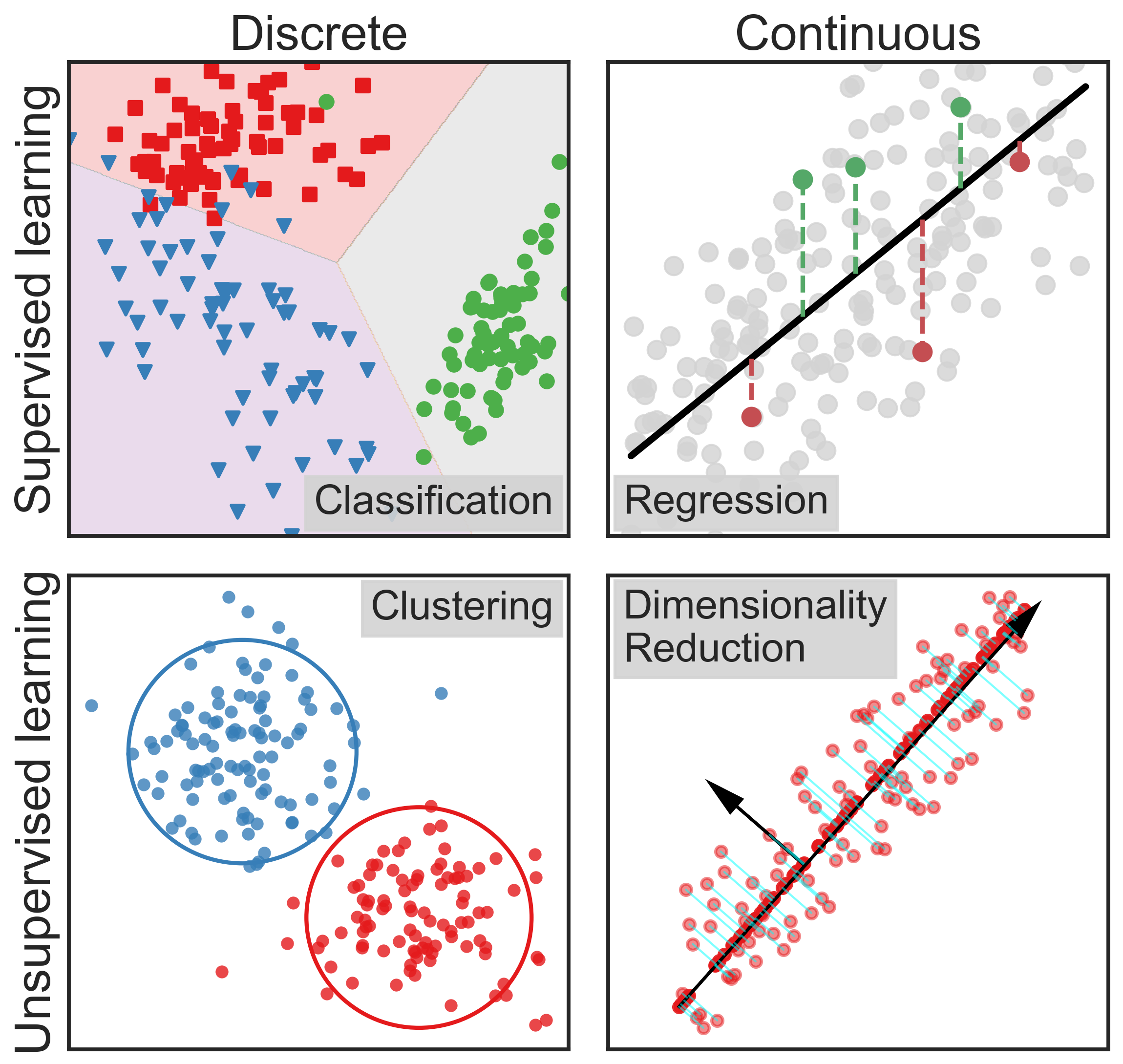
Categorizing Analytical Methods
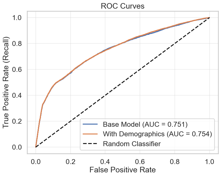
Lab 10 Recap
| Logit (Base) | Logit (With Char) | OLS (Base) | OLS (With Char) | |
|---|---|---|---|---|
| (1) | (2) | (3) | (4) | |
| Intercept | -0.818*** | -0.832*** | 0.279*** | 0.278*** |
| credit_limit | -0.221*** | -0.229*** | -0.026*** | -0.027*** |
| last_payment_portion | -0.143*** | -0.136*** | -0.026*** | -0.026*** |
| no_activity_this_month | 0.036 | 0.056 | 0.010 | 0.012 |
| num_recent_payments | -0.133*** | -0.134*** | -0.018*** | -0.018*** |
| outstanding_balance | 0.115*** | 0.119*** | 0.011*** | 0.011*** |
| pay_this_month | 1.088*** | 1.085*** | 0.223*** | 0.222*** |
| gender[male] | 0.140*** | 0.020*** | ||
| marital_status[married] | 0.018 | 0.002 | ||
| marital_status[single] | -0.159 | -0.022 | ||
| education[2-university] | 0.050 | 0.006 | ||
| education[3-trade school] | -1.222*** | -0.105*** | ||
| education[4-graduate school] | 0.038 | 0.003 | ||
| education[5-phd] | -1.470*** | -0.133*** | ||
| age_decile[30] | -0.019 | -0.003 | ||
| age_decile[40] | 0.074 | 0.010 | ||
| age_decile[50] | 0.077 | 0.012 | ||
| age_decile[60] | 0.164 | 0.025 | ||
| age_decile[70] | 0.363 | 0.058 |
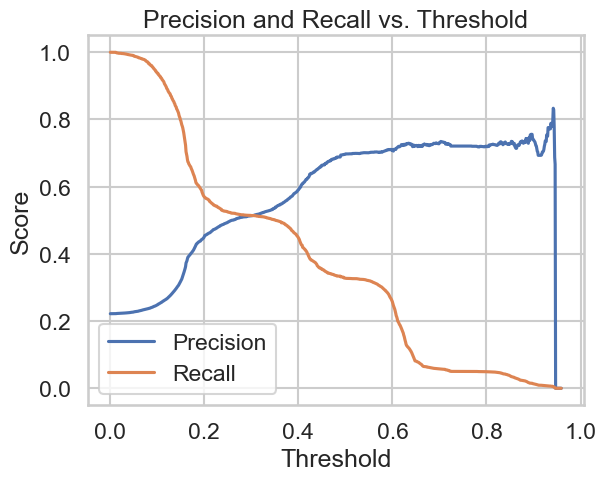
Precision and Recall
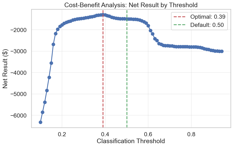
Expected Cost
Why unsupervised?
- Supervised learning is great at predicting what we want to know
- What if we don’t know what we don’t know?
- Are there customer “types” that we should be aware of
- What information is in text disclosures?
Analogy – Sorting Skittles
- A bag of skittles is dumped on the floor, and all measurements taken (color, size, location, etc.)
- Clustering – separate skittles into colors
- Dimensionality Reduction – first “factor” is color, then location, no difference in size
What is clustering?
- Separate data into different types or groups
- Similar to each other
- Different from other clusters
Clustering in Accounting
- Example: grouping transactions into types
- Classification might predict which account applies
- Clustering might find non directly labeled clusters such as “discretionary”, “periodic”, “abnormal”, etc.
- Clusters could capture factors that span accounts, but have similar features that may be worth monitoring
General approaches
- Centroid approach – clusters have “centers” and your assigned cluster is the closest one
- Density approach – clusters are concentrations of observations, like cities are densely populated areas
- Hierarchical approach – clusters form a hierarchy, like a tree diagram
Centroid Workhorse – K-means
- Approach:
- Choose K random cluster centers, assign every point to its nearest cluster
- Recompute the center of each cluster as center of its points, re-assign clusters to each point
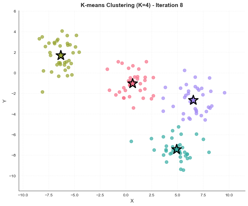
- Repeat #2 until there is no more movement
- Choosing K and the initial centers impact result
4-Means Example
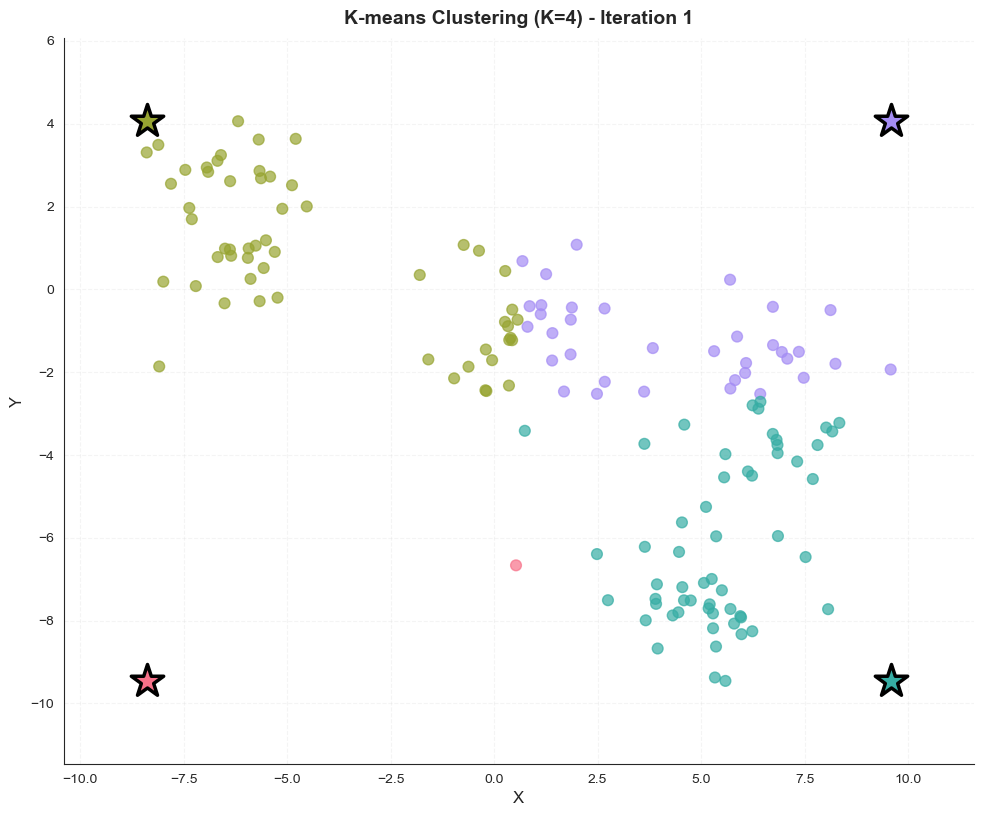
4-Means Example
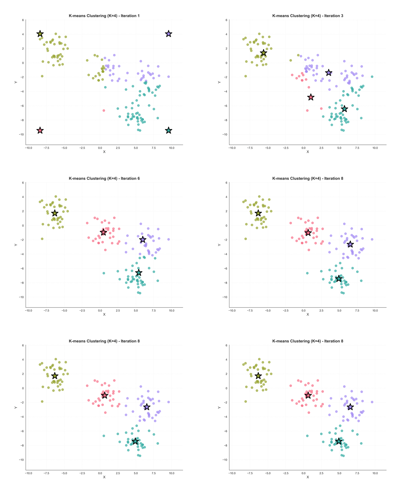
4-Means Example
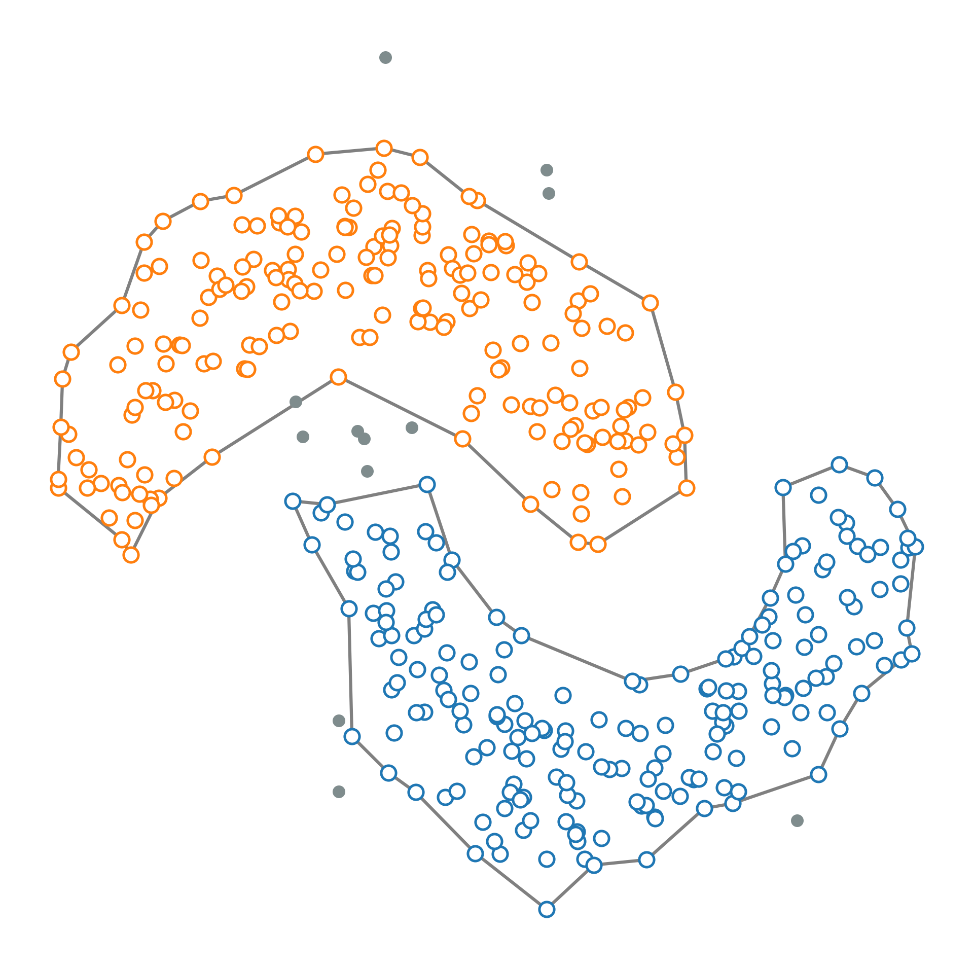
Density Clustering
- Connects areas of “high density” into clusters
- Discovers # of clusters
- Outliers in no cluster (good for anomaly detection)
- Like cities, hard to draw boundaries, hard to compare NYC and Moab
Hierarchical Clustering
- Determines a hierarchy by:
- Splitting dataset – top down
- Combining points – bottom up
- A cluster distance can be set to get N clusters at that point
- Smaller distance more clusters
- Good for hierarchical data
Example 1: Anomaly & fraud detection
- We may have some known cases of errors or fraud
- Could train a classifier to predict those, look for other similar cases
- What about future fraud?
- Bad actors are likely always looking to change their tactics, so backward looking methodology may fall short
Clustering transactions
- What if we clustered transactions on all available transaction characteristics (often, more is better)
- Look into outliers, observations that don’t fit
- Point anomaly: observation that always stands out
- Contextual anomaly: observation that stands out given some context, or expectations
- Collective anomaly: collection of observations that stand out because of their relation and characteristics
Approach to anomaly detection
- Perform clustering to set a “baseline” of normal (or the vast majority) of the data
- Determine what “outlier” means given this baseline
- Need some measure how far “out” an observation is (e.g., distance from the center of the cluster)
- Set a cutoff past which an observation is flagged
- Identify outliers, and look into them further (i.e., audit by exception)
clustering Value Add
- Historically fraud detection was rule based
- E.g., low income, high consumption/bank activity
- Clustering analyzes lots of variables simultaneously
- Identified outliers will have some complex interaction of variables that makes them unlike their peers
- Past some set of “rule of thumb” approaches, this kind of high dimensional rule making is hard for humans to do
Example 2: Customer Segmentation
- Classification needs some label to predict
- What are the labels for customer “types”?
- Clustering would provide groups
- Up to analyst to interpret groups, e.g. “high volume, prompt payer” and “high churn, low value”
- Starting conditions, model selection dictate value of identified clusters
- Compute is cheap!
Usefulness of Customer Clusters
- Identify factors associated with customer types that might have been hard to disentangle otherwise
- Learn new things about customer behavior patterns
- Resource allocation – pursue customer types that provide high value
- Risk identification – learn what correlates with risky type customers, to hedge or avoid
What is Dimensionality Reduction?
- Dimensionality reduction collapses many variables into just a few variables that capture the pertinent information
- Curse of dimensionality is when too many variables make analysis difficult, computationally infeasible, and more noise than signal
Accounting is Dimensionality Reduction
- Accounting takes thousands to millions of transactions and reduces them to 10-20 numbers on a balance sheet / income statement
- How we do this is based on a complex transformation function (called GAAP)
- The resultant 10-20 numbers each capture different aspects of the underlying high dimensional data, without losing anything important
Example – Kermit the Accountant
Example – Images
Dimensionality Reduction in Accounting
- Example: deriving customers risk “factors”
- Regression might predict probability of bad debt
- Dimensionality reduction might find risk “factors”, such as financial stability, risk appetite, loyalty, etc.
- Factors aid in understanding customer types, such as the stable risk seeker, or safe loyal customer, and can be used to decide services provided or AR terms
Principal Component Analysis
- The OLS of dimensionality reduction
- For N variables, PCA calculates up to N components
- First component explains the most variance
- Second component explains the next most, etc.
PCA Example on 2 variables
PCA Example on 4 variables
PCA Example on 4 variables
PCA Example on 4 variables
PCA Limitations
- PCA is a linear combinations of underlying variables, interpreting that result is not always straight forward
- Not using all N components will lose information
- Tradeoff # dimensions vs how much information kept
- Assumes linearity
Alternatives to PCA
- t-SNE: non-linear technique for visualization to represent high-dimensional clusters in 2D
- UMAP: non-linear technique that preserves the “geometric” structure of high-dimensional data
- Generally, non-linear approaches try to model the relationship between data, preserving what’s informative/repeated, dropping the rest
Autoencoders
- Take some data, throw it into a neural network, train it to predict itself
- If you squish the “middle” of the network enough, it has to learn how to re-generate the data without memorizing it
- That middle bit becomes a reduced dimensional representation of your input
Autoencoder


- math
- math
- 890 K
- 1,449 K
- 1,449 K
Dimensionality Reduction as First Step
- Some models based on distance (e.g. KNN) perform more poorly as number of features increases
- Applying dimensionality reduction first limits the dimensions to the most informative combinations
- Makes calculations possible
- Lessens risk of over-fitting
Visualization of myriad variables
- The interactions between variables is easy to observe “pair wise” in a pair plot, but not 3D+
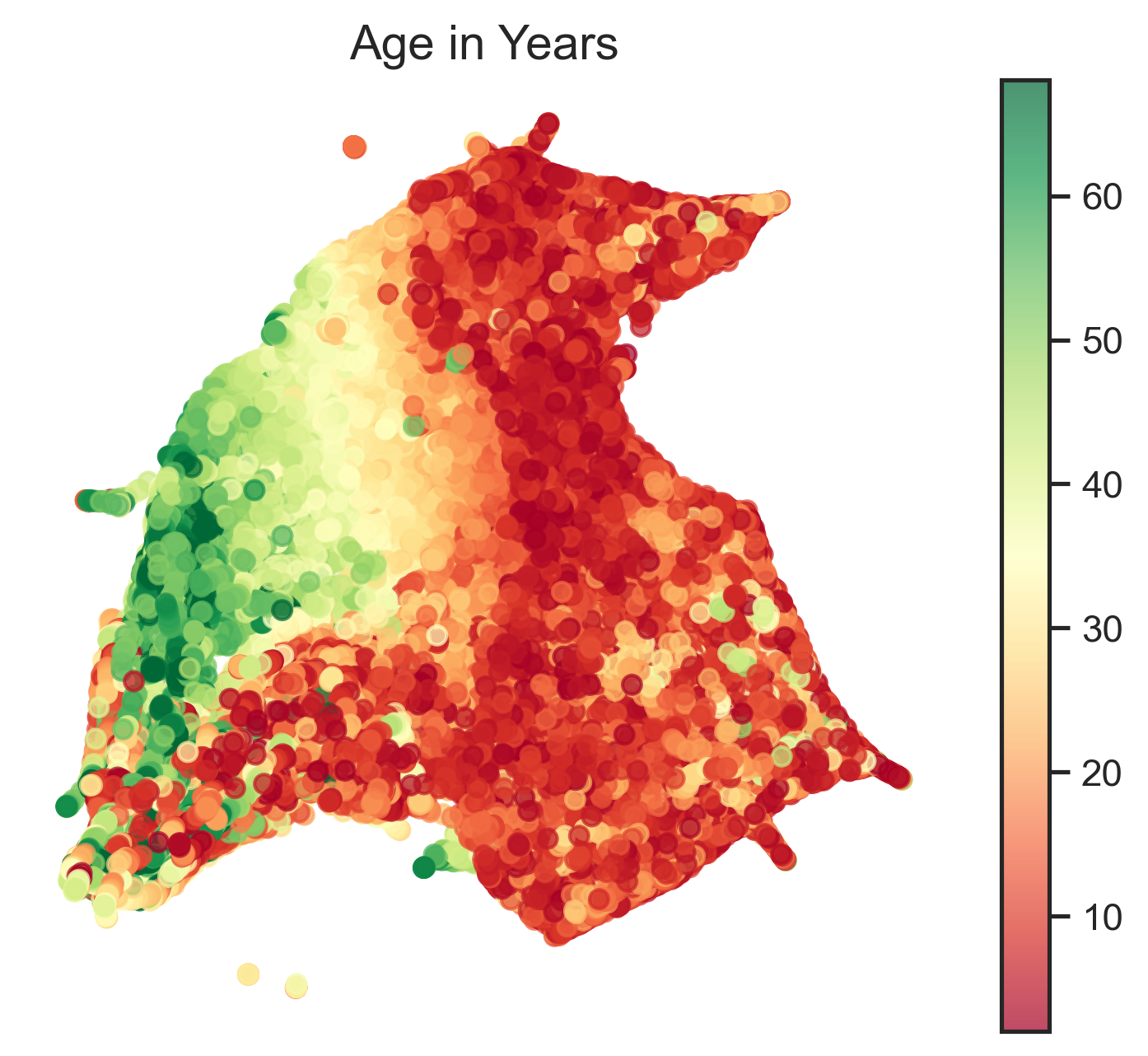
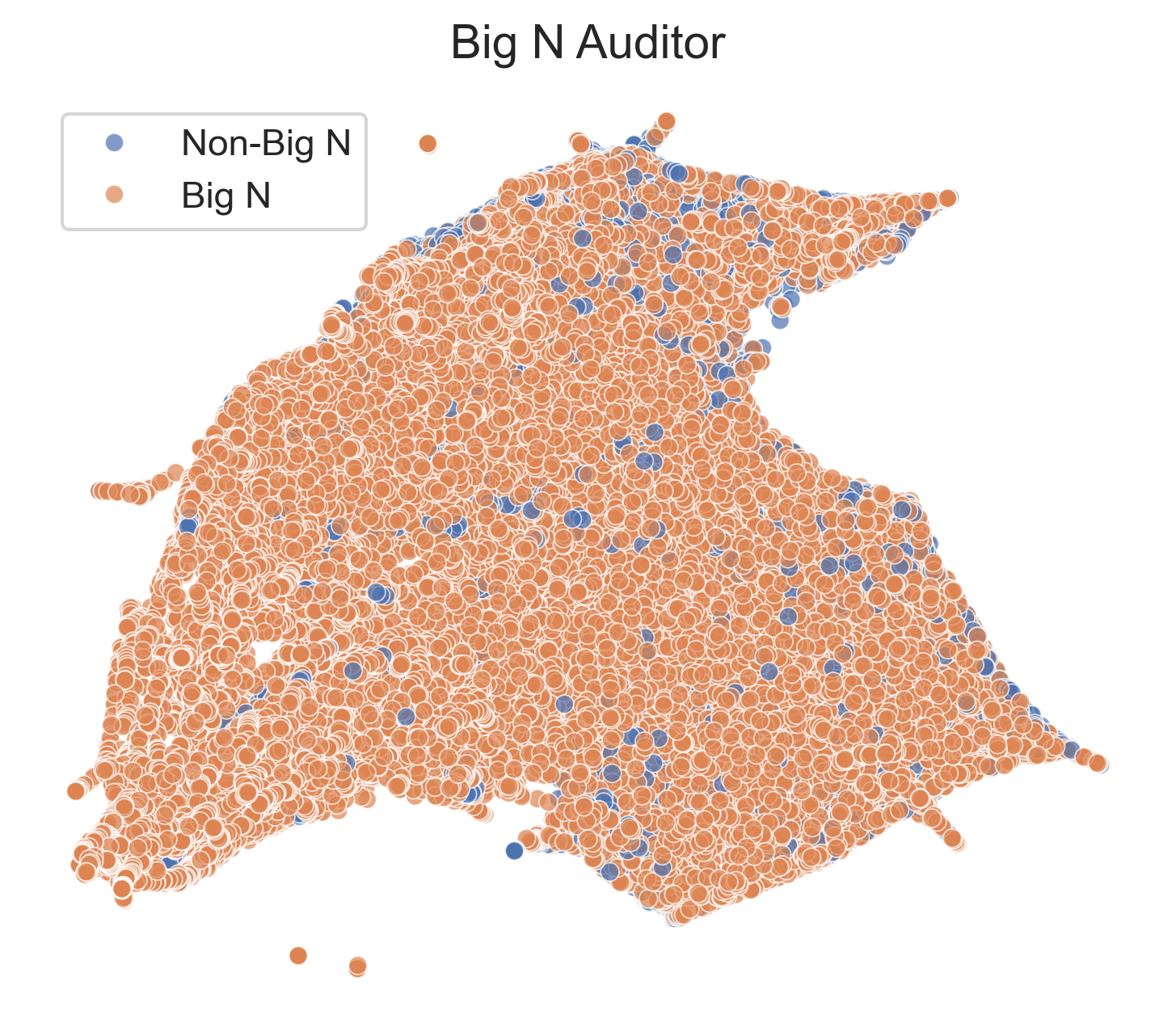
- PCA, t-SNE, UMAP, etc. preserve “structure” in the dataset, allowing for visual observation of clusters and other relationships in 2D that represent 3D+
FSA Ratio Example
- Performed UMAP on all accounting variables and FSA ratios from Project 1
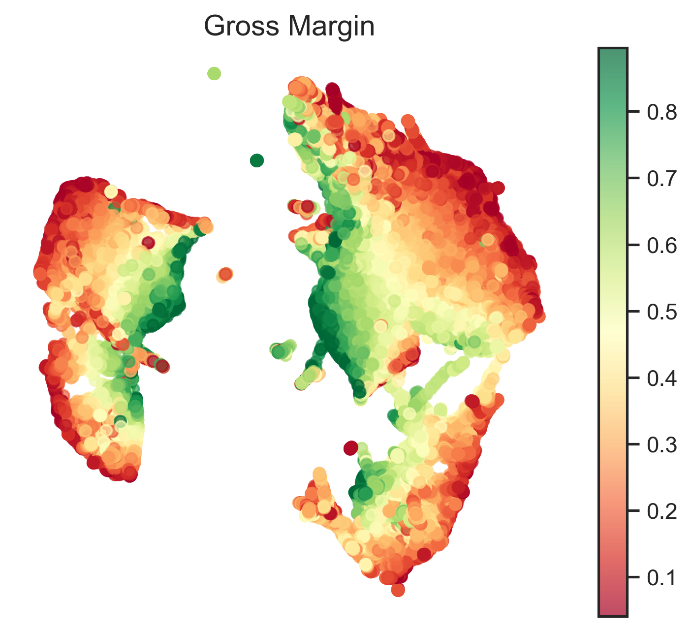
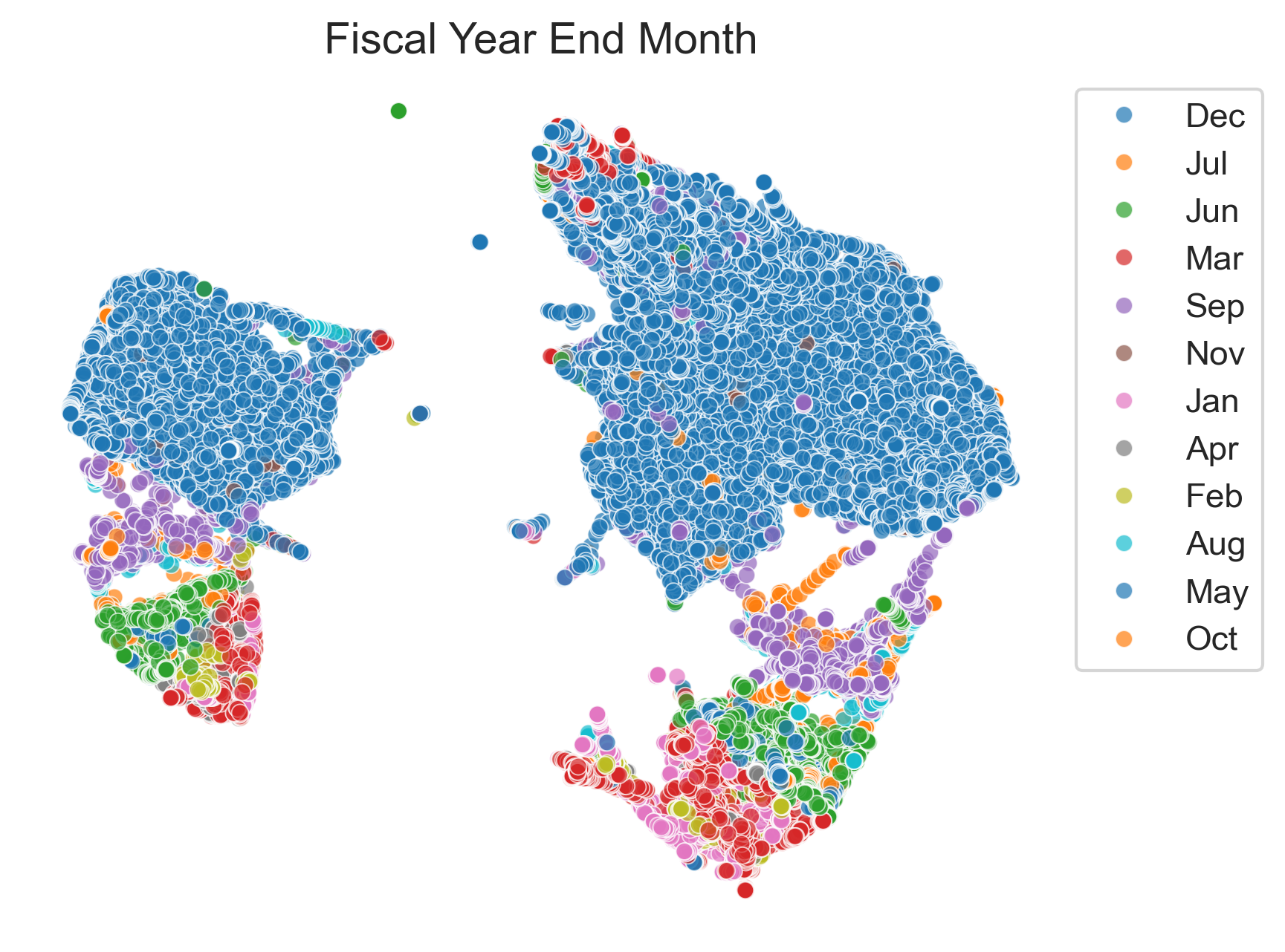
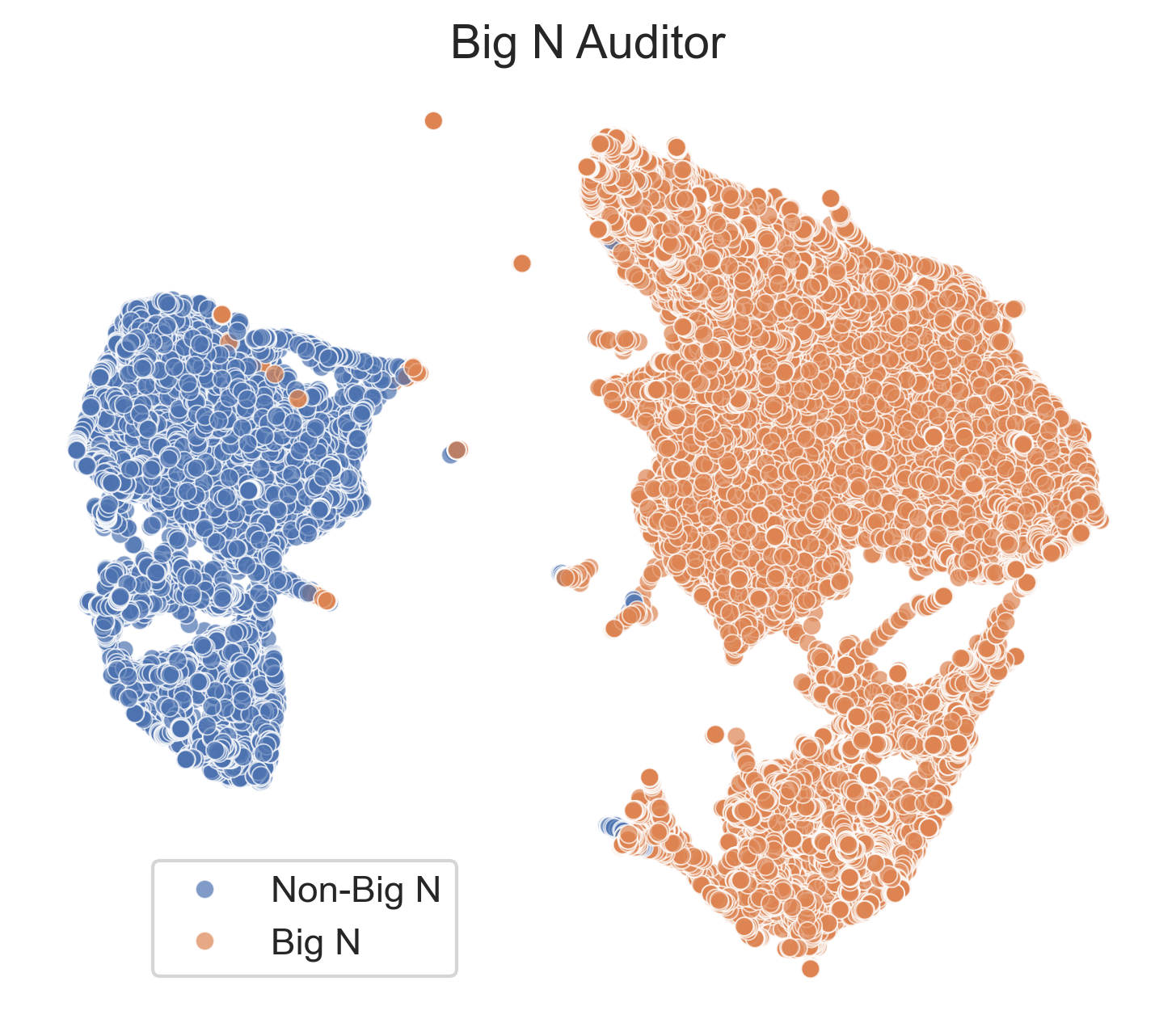
FSA Ratio Example – dropping big n
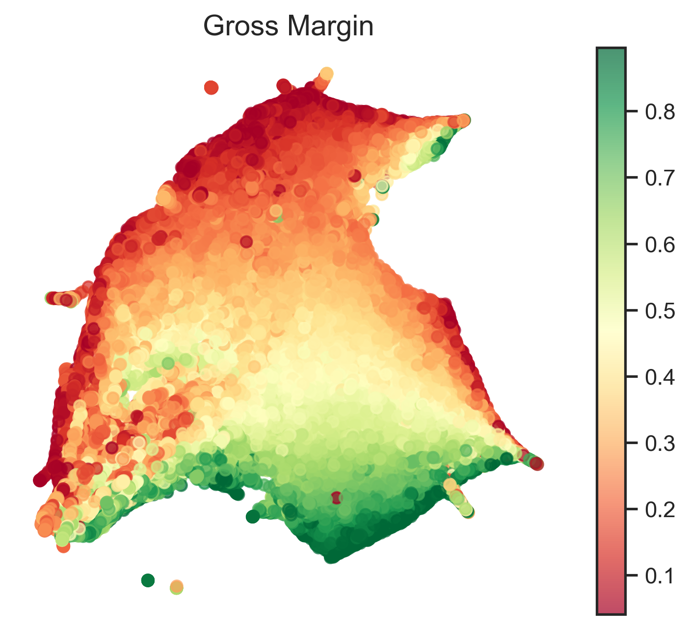
Textual Analysis
- Textual analysis is almost all dimension reduction
- Sentiment analysis reduces text to 2 dimensions
- Topic analysis discovers useful # of (few) dimensions
- LLM summarization as dimensionality reduction
- Typically a precursor to some subsequent use of the reduced dimensions
- E.g. supervised learning or clustering
Coming Up
- No Lab Wednesday, instead a work-session
- Project 3 due Sunday
- Project 4 due April 19 (right before Week 15)
- Presentations in class Week 15