Lab 9: Regression Modeling
Lab 9 introduces you to building, interpreting, and evaluating regression models for cost estimation. This lab builds on Lab 8’s exploration of relationships (R2) by having you actually construct descriptive models, interpret coefficients, and evaluate model performance using production cost data.
1. Assignment
Submission: To complete this lab, complete the Canvas quiz, including uploading screenshots and reporting results:
- Simple Volume Model: Regression of total cost on production volume with coefficients, significance, and R2
- ABC Model: Regression of total cost on activity based cost (ABC) drivers (material, labor, machine hours, etc.) with comparison to volume-only model
- Volume with Quarter Fixed Effects: Regression of total cost on production volume, adding indicator variables for each quarter, with coefficient comparison to Exercise 1
- Out-of-Sample Validation: Train volume model on 2015-2022 data, apply to 2023-2024 data, and compare RMSE/MAE/MAPE between training and test sets
Generally, you will submit screenshots of your regression output and error metrics for the Lab assignment, while answers to the written questions for each exercise will be submitted as part of the Homework.
Note: This lab demonstrates a fundamental cost accounting principle: detailed cost driver analysis provides better predictions than simple volume-based costing. The skills you practice here, running regressions, interpreting output, and evaluating predictions, are essential for cost management and budgeting.
1.1. Learning Objectives
By the end of this lab, you will be able to:
- Build and estimate OLS regression models using production cost data
- Compare simple volume-based models with detailed cost driver models
- Interpret regression coefficients in cost accounting terms (economic magnitude and statistical significance), including fixed effects
- Calculate and interpret model evaluation metrics (RMSE-Root Mean Square Error, MAE-Mean Absolute Error, MAPE-Mean Absolute Percentage Error)
- Apply proper train/test splits to assess out-of-sample prediction accuracy
- Understand when detailed cost analysis provides value over simple volume approximations
- Apply regression analysis to cost management and budgeting decisions
1.2. Tools
As always, you can use whatever modality you are comfortable with, but I recommend using Python for this lab, as regressions are far easier there.
- Excel: Data Analysis ToolPak provides regression analysis with full output tables, or you can use the
LINESTfunction for more compact output - Python:
statsmodelslibrary provides formula-based regression interface, with well-formatted regression output
2. Data
The dataset for this lab contains simulated monthly production costs for a manufacturing operation from 2015-2024. The data tracks both total costs and the underlying cost drivers that generate those costs, allowing you to compare simple volume-based cost estimation with detailed activity-based costing approaches.
The dataset production_costs_daily.csv contains, at the daily level, the following variables:
date: Full date (YYYY-MM-DD format)year: Year (2015-2024)month: Month number (1-12)quarter: Quarter number (1-4)cpi: Consumer price index (base year 2015 = 1).volume: Number of units produced in the monthdm_cost: Direct material cost (dollars)dl_cost: Direct labor cost (dollars)voh_cost: Variable overhead cost (dollars)material_lbs: Pounds of raw material consumedlabor_hours: Direct labor hours workedmachine_hours: Machine hours used in productionnum_batches: Number of production batches (drives setup labor)num_inspections: Number of quality inspections performedfoh_setup: Fixed overhead for production setupfoh_inspection: Fixed overhead for quality inspectionfoh_material_handling: Fixed overhead for material handlingfoh_facility: Fixed overhead for facility costs (rent, utilities, etc.)foh_total: Total daily fixed overheadtotal_variable_cost: Total daily variable costtotal_cost: Total daily cost
2.2. Key Variables for This Lab
Outcome Variable (Y)
total_cost: Total monthly production cost (dollars)- Includes all direct materials, direct labor, variable overhead, and fixed overhead
- This is what we want to predict
Simple Model Predictor (X)
volume: Number of units produced in the month- Traditional volume-based costing uses this as the single driver
- Expected R2 ≈ 80% when predicting total_cost
Detailed Cost Driver Predictors (multiple Xs)
- Material drivers:
material_lbs: Pounds of raw material consumed
- Labor drivers:
labor_hours: Direct labor hours workednum_batches: Number of production batches (drives setup labor)
- Machine drivers:
machine_hours: Machine hours used in productionnum_inspections: Number of quality inspections performed
Expected improvement: Using detailed cost drivers should increase R2 from ~80% to ~90%, demonstrating the value of detailed cost analysis.
2.3. Significance Levels
When interpreting regression output, you may see multiple ways to assess statistical significance of coefficients:
- P-value: Probability of observing the data if the null hypothesis (coefficient = 0) is true
- Common thresholds: <0.05 (5%), <0.01 (1%)
- If p-value < threshold, reject null hypothesis and conclude coefficient is statistically significant
- T-statistic: Ratio of coefficient estimate to its standard error
- Higher absolute t-statistic indicates more evidence against null hypothesis
- Rough rule of thumb: |t| > 2 corresponds to p-value < 0.05
- Standard Error: Measure of uncertainty in coefficient estimate
- Smaller standard error relative to coefficient indicates more precise estimate
- Used to calculate t-statistic (t-statistic = coefficient / standard error)
Note: Be wary of over-reliance on statistical significance alone, for two reasons. Firstly, p-hacking is the practice of manipulating data or models until you achieve statistically significant results. So unless you did the analysis yourself, you should be cautious in interpreting the results of “significant” findings, especially with p-values close to 0.05 (i.e. t-statistics close to 2). Secondly, a coefficient can be statistically significant but economically meaningless if its magnitude is very small. Always interpret coefficients in business terms, considering both significance and practical impact.
3. Step-by-Step Instructions
This lab walks you through some important regression modeling concepts using production cost data. The homework will continue with year fixed effects, and then CPI adjustment.
Generally, when reporting the output of a regression model, you should include:
- Intercept and coefficients
- Standard errors or t-statistics or P-values for significance testing
- R2 and, optionally, adjusted R2
- Number of observations
3.1. Exercise 1: Simple Volume-Based Model
Objective: Build a traditional volume-based cost model that predicts total cost using only production volume.
Most basic cost accounting systems use a traditional cost system that assumes one cost driver. This is easy to implement but ignores the complexity of how different activities drive different costs. In this example, our traditional cost system assumes that total costs are a linear function of production volume (units produced).
3.1.1. Tasks
- Load the dataset: all years 2015-2024
- Run the regression: Use OLS (Ordinary Least Squares) regression
- Outcome variable (Y):
total_cost - Predictor variable (X):
volume
- Outcome variable (Y):
- Report the results: Take a screenshot of your regression output
- Calculate error metrics:
- Use the regression coefficients to calculate predicted values:
total_cost_hat - Calculate residuals:
residual = total_cost - total_cost_hat - Calculate RMSE:
sqrt(mean(residual^2)) - Calculate MAE:
mean(abs(residual)) - Calculate MAPE:
mean(abs(residual / total_cost)) * 100
- Use the regression coefficients to calculate predicted values:
3.1.2. Questions to Answer
- What is the coefficient on
volume? In cost accounting terms, what does this represent? - What is the intercept? What does this represent in cost accounting terms?
- What are the RMSE and MAE? How should you interpret these dollar values? Why is RMSE typically larger than MAE, and what does the magnitude of the difference tell you about the presence of large prediction errors? Which metric would you prefer to use when communicating results, and why?
- What is the MAPE? How should you interpret this value? Is it more or less useful than RMSE/MAE when communicating results?
3.2. Exercise 2: ABC (Activity-Based Costing) Model
Objective: Build a comprehensive cost model using detailed cost drivers to predict total cost more accurately than the simple volume model.
Activity-Based Costing (ABC) recognizes that different activities consume different resources. Instead of assuming all costs are driven by one cost driver (e.g., volume), ABC identifies specific cost drivers for each activity.
3.2.1. Tasks
- Load the dataset: all years 2015-2024
- Run the regression: Use OLS (Ordinary Least Squares) regression
- Outcome variable (Y):
total_cost - Predictor variables (X):
material_lbs,labor_hours,machine_hours,num_batches,num_inspections
- Outcome variable (Y):
- Report the results: Take a screenshot of your regression output
- Create comparison table:
| Metric | Volume Only (Ex 1) | ABC Model (Ex 2) |
|---|---|---|
| R2 | ||
| RMSE | ||
| MAE | ||
| MAPE (%) |
3.2.2. Questions to Answer
- How much did R2 improve from the volume-only model to the ABC model? What does this tell you about the value of detailed cost analysis?
- What is the coefficient on
labor_hours? In cost accounting terms, what does this represent? - What is the coefficient on
material_lbs? In cost accounting terms, what does this represent? - Which cost drivers are statistically significant at the 5% level? What does this tell you about which activities are important in driving total costs?
3.3. Exercise 3: Volume with Quarter Fixed Effects
Objective: Improve the simple volume model by controlling for seasonal patterns using quarter indicator variables (i.e., quarter fixed effects).
Production costs could vary by season due to factors like heating/cooling costs, holiday staffing/overtime, or seasonal demand patterns. Fixed effects allow each quarter to have its own baseline cost level while maintaining the same volume-cost relationship. Note: it’s worth mulling over how these quarter fixed effects, which allow the intercept to vary by quarter, differ from allowing the slopes to vary by quarter (which technically would be an interaction between the quarter indicators and the volume variable).
3.3.1. Tasks
- Load the dataset: all years 2015-2024
- Create quarter indicator variables:
- Quarter 2 indicator: 1 if
quarter == 2, 0 otherwise - Quarter 3 indicator: 1 if
quarter == 3, 0 otherwise - Quarter 4 indicator: 1 if
quarter == 4, 0 otherwise - Important: Do NOT create a quarter 1 indicator (this avoids multicollinearity)
- Quarter 2 indicator: 1 if
- Run the regression: Use OLS regression
- Outcome variable (Y):
total_cost - Predictor variables (X):
volume, Q2 indicator, Q3 indicator, Q4 indicator
- Outcome variable (Y):
- Report the results: Take a screenshot of your regression output
- Compare to Exercise 1:
| Metric | Volume Only (Ex 1) | Volume + Quarter FE (Ex 3) |
|---|---|---|
| R2 | ||
| RMSE | ||
| MAE | ||
| MAPE (%) |
3.3.2. Questions to Answer
- Verify that the coefficient on
volumebasically did not change when you added quarter fixed effects. What does this mean economically? - Why do we only include 3 quarter indicators instead of 4? What does the intercept represent in this model?
- Which quarter has the highest baseline costs (holding volume constant)? Which has the lowest? Note: consider your answer to the question above!
- Are the quarter effects statistically significant? What does this tell you about seasonal patterns in production costs?
3.4. Exercise 4: Out-of-Sample Validation
Objective: Assess model performance using a train/test split to evaluate out-of-sample prediction accuracy.
The real test of a cost model is out-of-sample performance, or how well it predicts future costs that weren’t used to train the model. This is critical for budgeting: you build a cost model using historical data, then use it to forecast future period costs.
3.4.1. Tasks
- Split the data:
- Training set:
year < 2023(8 years of historical data) - Test set:
year >= 2023(most recent 2 years) - Note: You can split the data into separate datasets, or simply filter out the test years when training the model
- Training set:
- Train the volume model on training data only:
- Outcome variable (Y):
total_cost - Predictor variable (X):
volume
- Outcome variable (Y):
- Make predictions on both train and test sets:
- Apply model coefficients to both training data and test data to calculate
total_cost_hatacross all years - Calculate residuals for all years:
residual = total_cost - total_cost_hat
- Apply model coefficients to both training data and test data to calculate
- Calculate error metrics:
- Calculate RMSE, MAE, MAPE separately for training and test sets
| Dataset | RMSE | MAE | MAPE (%) | # Observations |
|---|---|---|---|---|
| Training (2015-2022) | ||||
| Testing (2023-2024) |
3.4.2. Questions to Answer
- How did RMSE for the test set compare to training set RMSE? What does this tell you about model performance on new data?
- How did the in-sample MAPE (i.e., for the training data) compare to the in-sample MAPE from Exercise 1 (note, this is the exact same model as Exercise 1, just trained on all but the last 2 years of data)? What do you think is happening here?
- What is the MAE for the test set, in plain English? For example, “On average, monthly cost predictions for 2024 were off by $____”
- What is the MAPE for the test set, in plain English? For example, “On average, monthly cost predictions for 2024 were off by ____%“
4. Cost Accounting Insights
This lab demonstrates several important cost accounting principles:
Volume-Based Costing vs. Activity-Based Costing:
| Approach | Complexity | Accuracy | When to Use |
|---|---|---|---|
| Volume-Based (Exercise 1) | Low - only tracks production volume | Moderate (R2 ≈ 80%) | Simple products, limited overhead, quick estimates |
| Activity-Based (Exercise 2) | High - tracks multiple cost drivers | High (R2 ≈ 90%) | Complex processes, significant overhead, pricing decisions |
| Volume + Quarter FE (Exercise 3) | Low-Medium - tracks volume + seasonality | Moderate (R2 ≈ 80%) | When seasonal patterns are important |
Intended Takeaways:
- ABC drivers provide improvement over simple volume-based costing (~10% R2 increase in this dataset)
- Quarter fixed effects capture seasonal patterns but add less predictive power than ABC drivers
- Out-of-sample validation is critical for assessing real-world model performance
Practical Applications:
- Budgeting: Build cost models from historical data, predict future period costs
- Pricing: Understand true marginal costs to inform pricing decisions
- Process Improvement: Identify which cost drivers have biggest impact on total cost
- Variance Analysis: Compare actual costs to model predictions, investigate significant deviations
- Model Validation: Use train/test splits to assess real-world prediction accuracy
5. Technical Guidance
This section provides step-by-step instructions for implementing the lab exercises in your tool of choice.
5.1. Excel Implementation
5.1.1. Running Regressions in Excel with Data Analysis ToolPak
- Go to Data → Data Analysis → Regression
- If you don’t see “Data Analysis”, enable it:
- Windows: File → Options → Add-ins → Analysis ToolPak
- Mac: Tools → Add-ins → Analysis ToolPak
- If you don’t see “Data Analysis”, enable it:
- Set Input Y Range: Select
total_costcolumn (including header) - Set Input X Range: Select
volumecolumn (including header)- You can select multiple columns side-by-side for multiple predictors, e.g. for Exercise 2.
- Check Labels (since you included headers)
- Choose Output Range (click on a cell where you want the output, or select “New Worksheet”)
- Check Residuals to get predicted values automatically (but note, this won’t give you residuals for out-of-sample data, you’ll need to calculate those manually)
- Click OK
5.1.2. Running Regressions in Excel with LINEST Function
The LINEST function (documentation) provides a compact way to get regression coefficients and statistics. While it’s output is a bit more inscrutable than the Data Analysis ToolPak, it can be far easier to use just a single excel formula instead of clicking through menus.
- Make your data a table (ctrl/cmd + T), for far easier range selection. Let’s assume your table is named
Table1(which it would be by default). - Enter the following formula:
=LINEST(Table1[total_cost], Table1[volume], TRUE, TRUE)- To select multiple columns, it would be:
=LINEST(Table1[total_cost], Table1[[material_lbs]:[num_inspections]], TRUE, TRUE)
- To select multiple columns, it would be:
- Press Enter
- On some versions of Excel, you might have to press Ctrl + Shift + Enter to enter as an array formula. Try just hitting Enter first, and if it doesn’t work, try the array formula method.
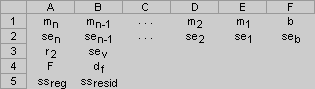
- The output will be a 5-row by N-column array, where N is the number of predictors plus one (for intercept). The rows contain:
- Row 1: Coefficients (intercept last, then predictors in reverse order. Totally logical and straightforward. Duh.)
- Row 2: Standard errors
- Row 3: R Square, Standard Error of Y estimate, F statistic, Degrees of Freedom
- Row 4: Regression SS, Residual SS, Total SS
- Row 5: Regression MS, Residual MS, F statistic again
- Diagram from MS support documents:
5.1.3. Creating Quarter Indicator Variables
To create indicators in Excel, create one column for each unique value, then use an IF formula. Here’s how to create quarter indicators:
- Create new columns for Q2, Q3, Q4 indicators (note: no Q1 indicator)
- Q2 indicator formula (assuming your data is in a table):
- In a new column:
=IF([@quarter]=2,1,0) - Copy down for all rows (automatically done if you made your data a table)
- If you want to be fancy, you can use
=--([@quarter]=2)to get 1/0 directly
- In a new column:
- Q3 indicator formula:
=IF([@quarter]=3,1,0) - Q4 indicator formula:
=IF([@quarter]=4,1,0)
Tip: If you want to put these in the regression with your other predictors (e.g. volume), make sure all these columns are adjacent when selecting the Input X Range in the regression dialog. So that will mean making 3 new columns next to volume for Q2, Q3, Q4 indicators.
5.1.4. Calculating Error Metrics
The Residual Output gives you predicted values, but you need to calculate metrics manually. You also need to calculate residuals manually for out-of-sample data, so I will show you how to first calculate predicted values, then residuals, then metrics. The below also assumes you made your data a table for easy referencing, called Table1.
-
Calculate predicted values from any regression model:
- Create a new column, and let’s call it
total_cost_hat- TL;DR: hat indicates predicted value. If you’re curious, “hat” denotes predicted value because in statistics we write the predicted
yasŷ, and that little caret is called a “hat”. If you’re even more curious, that hat symbol is called a circumflex symbol (ˆ), and is an accent mark derived from the ancient Greek “perispōménē” and the Latin “circumflexus,” meaning “bent around”.
- TL;DR: hat indicates predicted value. If you’re curious, “hat” denotes predicted value because in statistics we write the predicted
- Assuming the intercept is in cell
AB2and volume coefficient is in cellAA2. - In the new column, enter
=$AB$2 + [@volume] * $AA$2- Note: If this new column is not in your table, you have to add the table reference manually:
= $AB$2 + Table1[@[volume]] * $AA$2, because in the same table, Excel assumes theTable1reference for you.
- Note: If this new column is not in your table, you have to add the table reference manually:
- The
$freezes the cell reference so it doesn’t change when you copy the formula down, and always points to the same coefficient. - Note 1: if you have multiple predictors, just add each of them in the same way:
= $AB$2 + [@material_lbs] * $AA$2 + [@labor_hours] * $Z$2 + ... - Note 2: You can copy this formula down the entire column, even when you have out-of-sample data. This is because you calculate predicted values out-of-sample using the model you fit with on your training data, but that’s just the coefficients you calculated in your regression (that’s what defines the “model”). In other words, the only thing changing when you calculate in-sample and out-of-sample statistics is which rows you include in your calculations.
- Create a new column, and let’s call it
-
Calculate residuals:
- Create a new column, call it
residuals - In the new column, enter
= [@total_cost] - [@total_cost_hat] - Note 1: Again, you can copy this formula down the entire column, even for out-of-sample data.
- Note 2: This will be the same no matter how many predictors you have, because the predictors just go into calculating the predicted value of total cost.
- Create a new column, call it
-
Calculate RMSE:
- In a cell:
=SQRT(AVERAGE(Table1[residuals]^2))- This cell should not be in/next to your table because this isn’t a whole column, and so you need the explicit
Table1reference
- This cell should not be in/next to your table because this isn’t a whole column, and so you need the explicit
- In a cell:
-
Calculate MAE:
- In a cell:
=AVERAGE(ABS(Table1[residuals]))
- In a cell:
-
Calculate MAPE:
- In a cell:
=AVERAGE(ABS(Table1[residuals]/Table1[total_cost]))*100
- In a cell:
-
Calculate metrics separately for train/test sets:
- You can use
FILTERfunction to filter rows by year (FILTER documentation) - For example, RMSE for training set (2015-2022):
=SQRT(AVERAGE(FILTER(Table1[residuals], Table1[year]<2023)^2))
- RMSE for test set (2023-2024):
=SQRT(AVERAGE(FILTER(Table1[residuals], Table1[year]>=2023)^2))
- Similarly for MAE and MAPE, just wrap the
ABSfunction in aFILTERfunction.- Note: just make sure the filter comes before any aggregation function like
AVERAGE(which is why outside theABSis fine). Example MAPE: `=AVERAGE(FILTER(ABS(Table1[residuals]/Table1[total_cost]),Table1[year]>=2023))*100
- Note: just make sure the filter comes before any aggregation function like
- You can use
5.2. Python Implementation
The following is example code for implementing the lab exercises in Python. You could think of each section as a cell in your colab notebook, but note that the code below doesn’t just copy/paste complete the Lab. It does, however, cover all the code you need to complete the exercises, you just have to duplicate and combine as needed for each exercise.
5.2.1. Setup and Data Loading
# Load Imports
import pandas as pd
import numpy as np
import statsmodels.formula.api as smf

df = pd.read_csv('production_costs_daily.csv', parse_dates=['date'])
# View first 2 rows
df.head(2)
5.2.2. Running a regression
Below is some example code for running models, and showing the output for the first exercise.
# Run simple regression: total_cost ~ volume
exercise1_volume_model = smf.ols('total_cost ~ volume', data=df).fit()
exercise2_abc_model = smf.ols('total_cost ~ material_lbs + labor_hours + machine_hours + num_batches + num_inspections', data=df).fit()

# Output regression output for submission screenshot
print(exercise1_volume_model.summary())
To include quarter fixed effects, you can either create indicator variables manually (like those Excel folk are doing as we speak), or, because Python is awesome, use the convenient syntax for making dummy variables: C(quarter). So that would look like:
smf.ols('total_cost ~ volume + C(quarter)', data=df).fit()I hope you start seeing how fantastic statsmodels is for regression work. And if you want to start making fancy tables with multiple models side-by-side, you can use the statsmodels summary_col function. Here’s a quick example:
from statsmodels.iolib.summary2 import summary_col
model_volume = smf.ols('total_cost ~ volume', data=df).fit()
model_abc = smf.ols('total_cost ~ material_lbs + labor_hours + machine_hours + num_batches + num_inspections', data=df).fit()
model_volume_qfe = smf.ols('total_cost ~ volume + C(quarter)', data=df).fit()
results_table = summary_col([model_volume, model_abc, model_volume_qfe],
                            stars=True,
                            model_names=['Volume Only', 'ABC Model', 'Volume + Q FE'],
                            info_dict={'R-squared': lambda x: f"{x.rsquared:.4f}",
                                       'Adj. R-squared': lambda x: f"{x.rsquared_adj:.4f}",
                                       'No. observations': lambda x: f"{int(x.nobs)}"})
print(results_table)
5.2.3. Error Calculations
This is Python, of course the calculations we need are already written up for us in some library. In this case, it’s sklearn.metrics. Note: sklearn is short for “scikit-learn”, a popular machine learning library in Python that includes many useful tools for model evaluation. Also note: yes, you can absolutely abuse sklearn for awesome.
from sklearn.metrics import mean_squared_error, mean_absolute_error, mean_absolute_percentage_error

# Calculate predictions and residuals, and put them in the dataframe
df['total_cost_hat_e1'] = exercise1_volume_model.predict(df)
df['residual_e1'] = df['total_cost'] - df['total_cost_hat_e1'] # not necessary

# Calculate error metrics
rmse_e1 = np.sqrt(mean_squared_error(df['total_cost'], df['total_cost_hat_e1']))
mae_e1 = mean_absolute_error(df['total_cost'], df['total_cost_hat_e1'])
mape_e1 = mean_absolute_percentage_error(df['total_cost'], df['total_cost_hat_e1']) * 100

print(f"\nIn-sample error metrics:")
print(f"RMSE: ${rmse_e1:,.2f}")
print(f"MAE: ${mae_e1:,.2f}")
print(f"MAPE: {mape_e1:.2f}%")
5.2.4. Train/Test Split
Conceptually, you could split your dataset into train/test sets by creating two separate dataframes. However, it’s often easier to just filter the dataframe when training the model, then use the same model to predict on the full dataset (both train and test). This is because the model coefficients are what define the model, and once you have those, you can apply them to any data.
# Train volume model on training data only
model_train = smf.ols('total_cost ~ volume', data=df[df['year'] < 2023]).fit()

# Make predictions on both train and test sets at once
df['total_cost_hat'] = model_train.predict(df)

# Calculate metrics for both datasets
def calc_metrics(df, actual='total_cost', predicted=None):
    if predicted is None: predicted = actual + '_hat'
    rmse = np.sqrt(mean_squared_error(df[actual], df[predicted]))
    mae = mean_absolute_error(df[actual], df[predicted])
    mape = mean_absolute_percentage_error(df[actual], df[predicted]) * 100
    return { 'RMSE': rmse, 'MAE': mae, 'MAPE': mape , 'N': len(df.dropna(subset=[actual, predicted]))}

# Training metrics
train_metrics = calc_metrics(df[df['year'] < 2023])

# Testing metrics
test_metrics = calc_metrics(df[df['year'] >= 2023])

# Print comparison table
pd.DataFrame([train_metrics, test_metrics], index=['Training (2015-2022)', 'Testing (2023-2024)'])
5.3. Common Issues and Troubleshooting
-
Problem: Excel “Regression” option not available in Data Analysis
- Cause: Analysis ToolPak not enabled
- Solution: File → Options → Add-ins → Manage Excel Add-ins → Check “Analysis ToolPak” → OK. On MacOS: Tools → Add-ins → Check “Analysis ToolPak” → OK
-
Problem: Excel won’t run regression with non-adjacent columns
- Cause: Input X Range must be contiguous columns
- Solution: Copy your predictor columns to new columns next to each other, then run regression
-
Problem: R2 is not around 80% for volume model or 90% for ABC model
- Cause: Using wrong variables or wrong dataset
- Solution: Verify you’re using
total_costas outcome variable, and correct predictors
-
Problem: Negative coefficients on cost drivers
- Cause: If predictor is insignificant, random noise could make it negative
- Solution: Ignore it, insignificance has an economic meaning (no relationship)
-
Problem: Test set error much higher than training set error
- Cause: Model overfitting and/or conditions changed in test period
- Solution: This can happen. If it were real-world data, you would document the degradation and consider possible explanations (inflation spike, supply chain disruption, etc.)