Week 9
Regressions
- Instructors
- Maclean Gaulin
Regressions
- A model predicting something we already know
- Diagnostic: understand why something happened
- Predictive: what we know helps forecast the future
- Requires us to have data on the outcome that we wish to predict (supervised learning)
- This is called “labeled” data; the outcome is the “label”
- Label = f(Features)
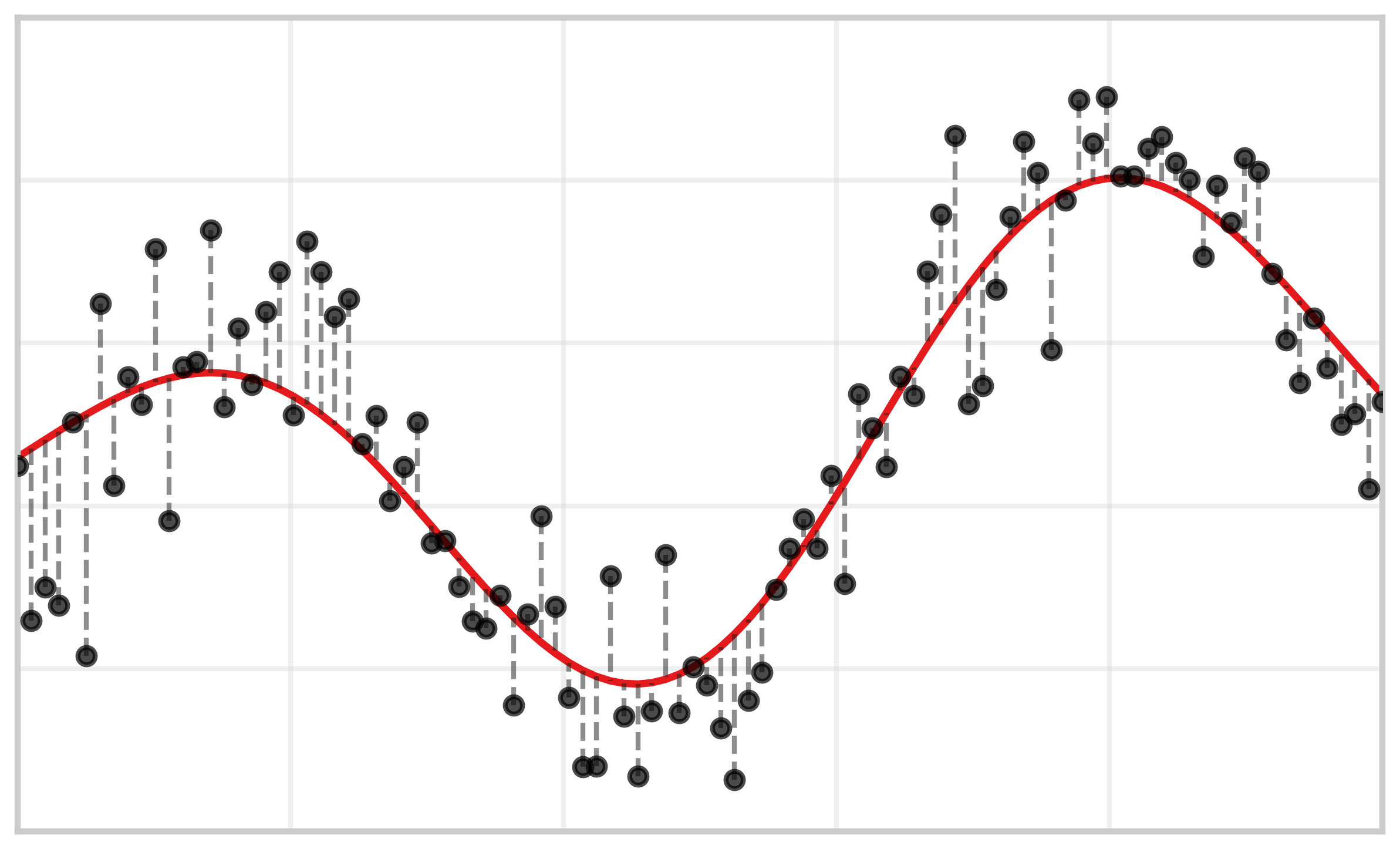
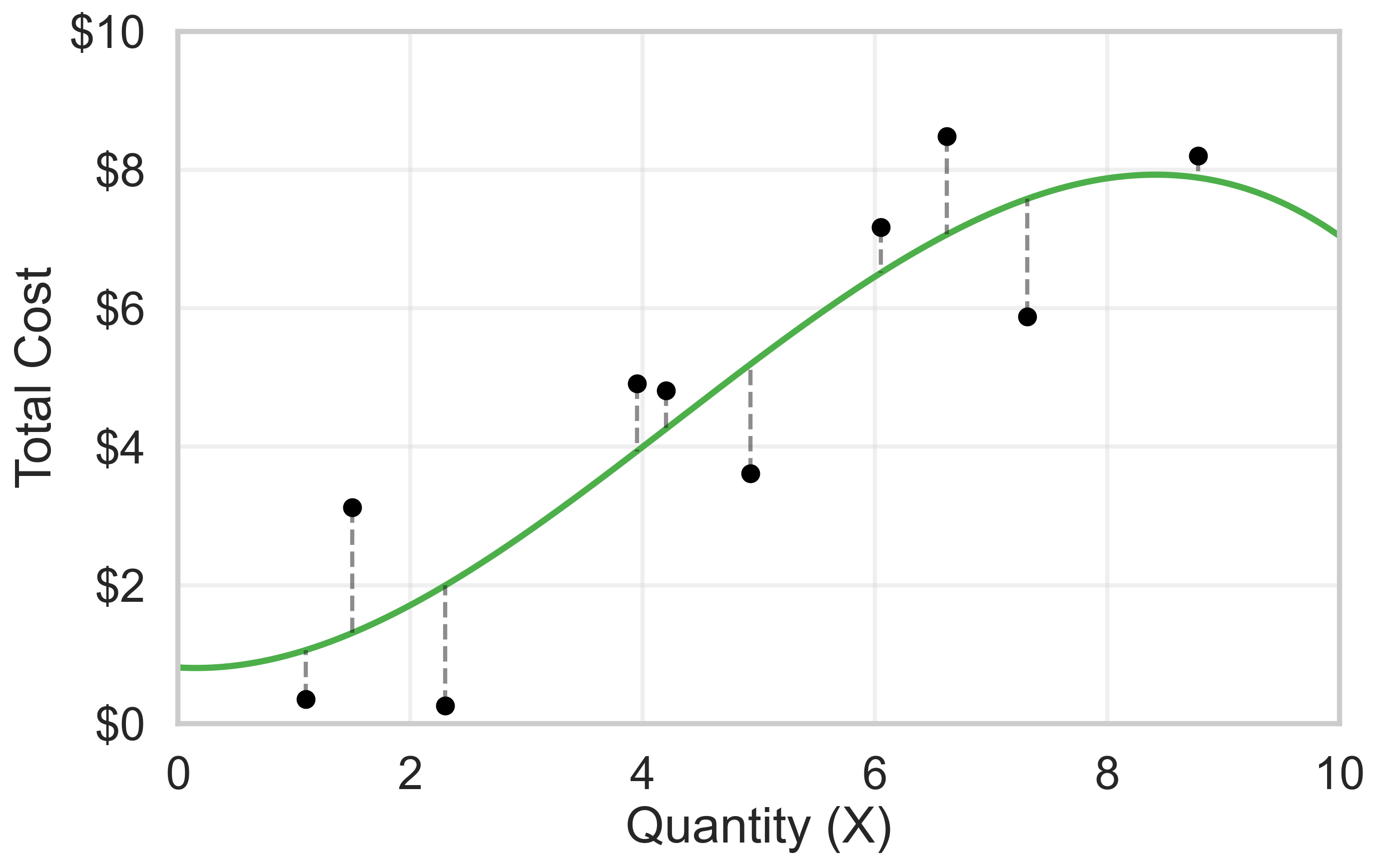
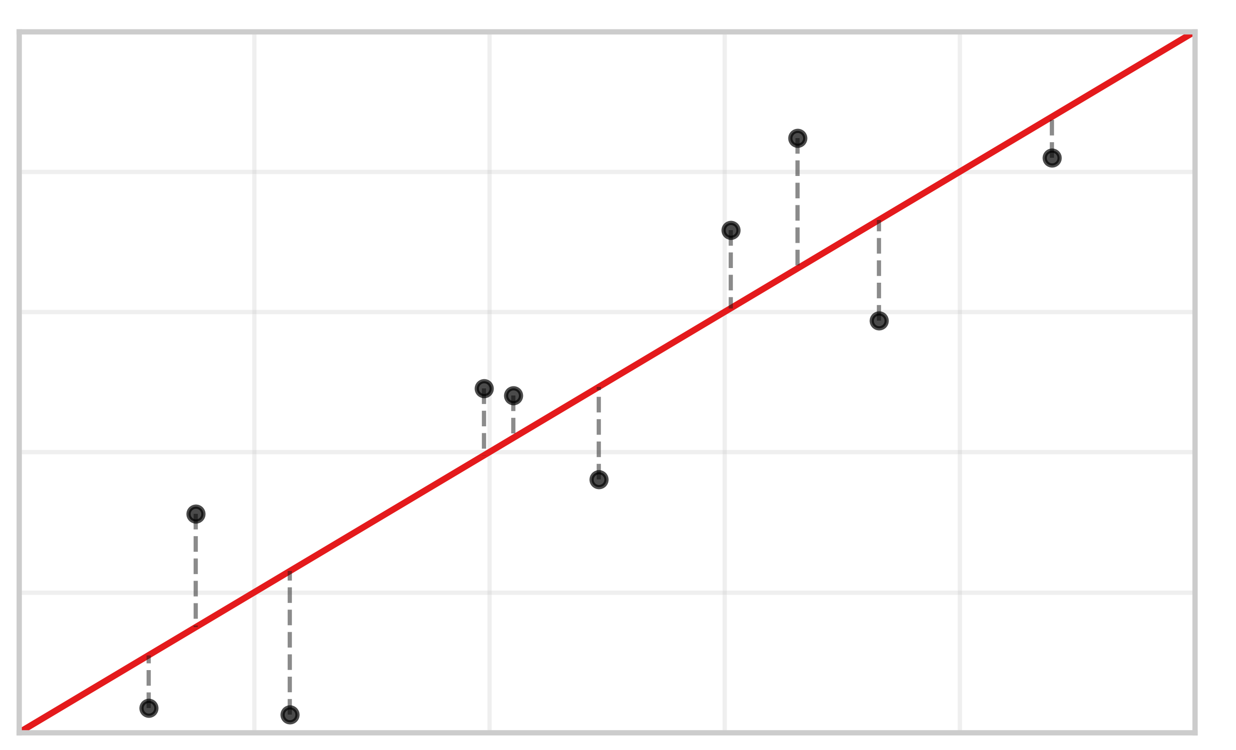
Regressions just fit a line
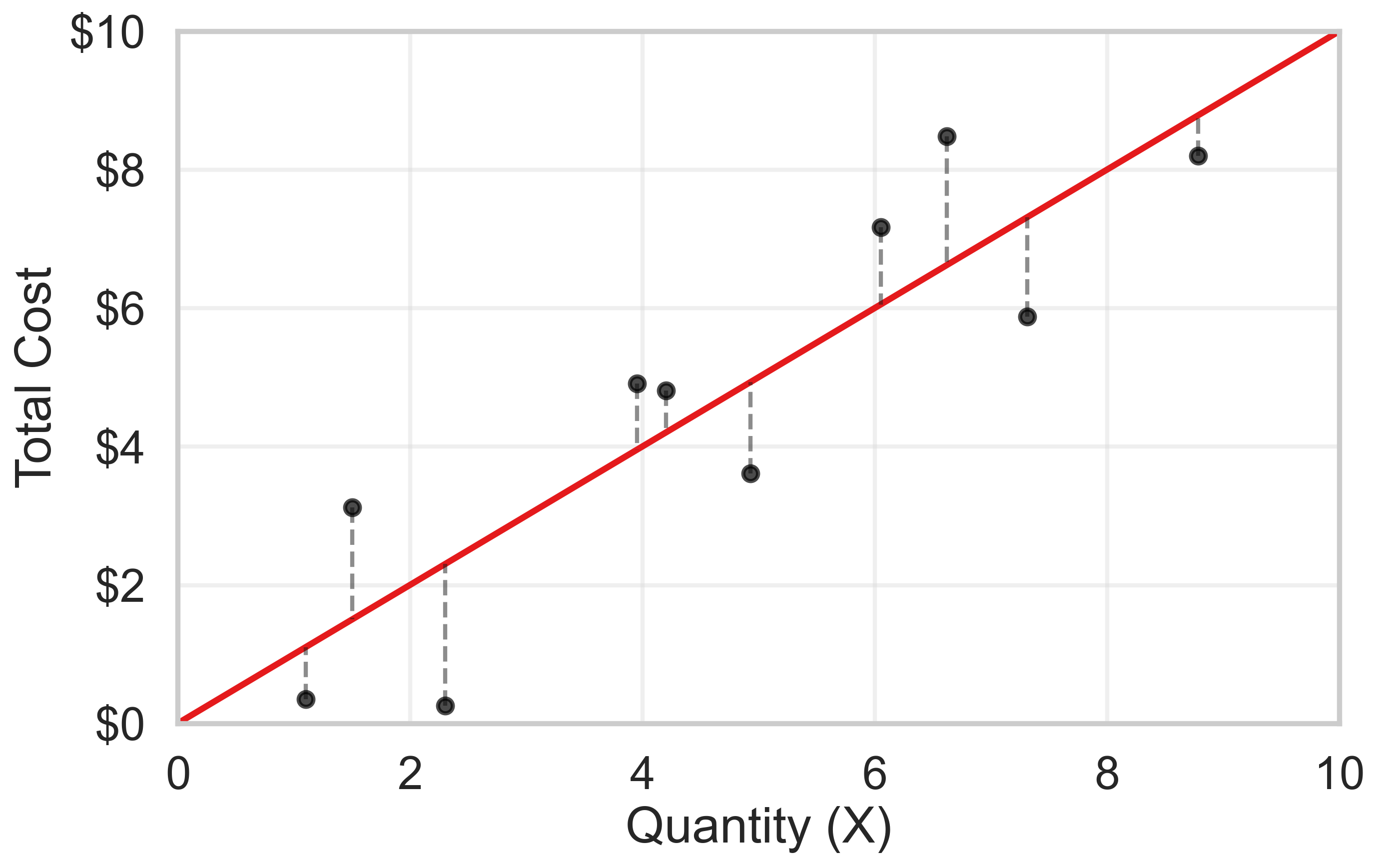
The dotted lines are the “error”
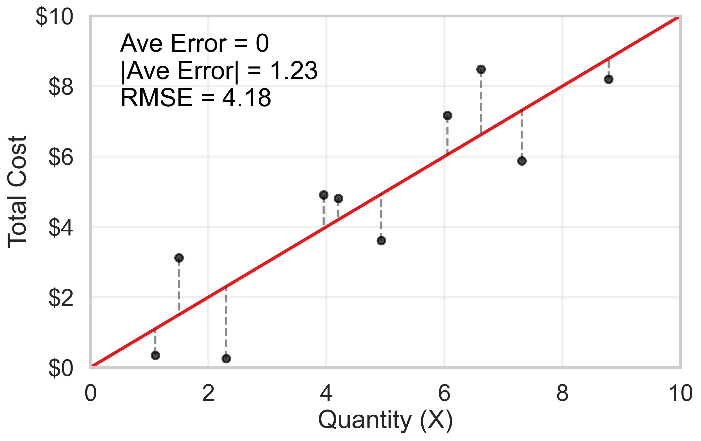
Could be any line
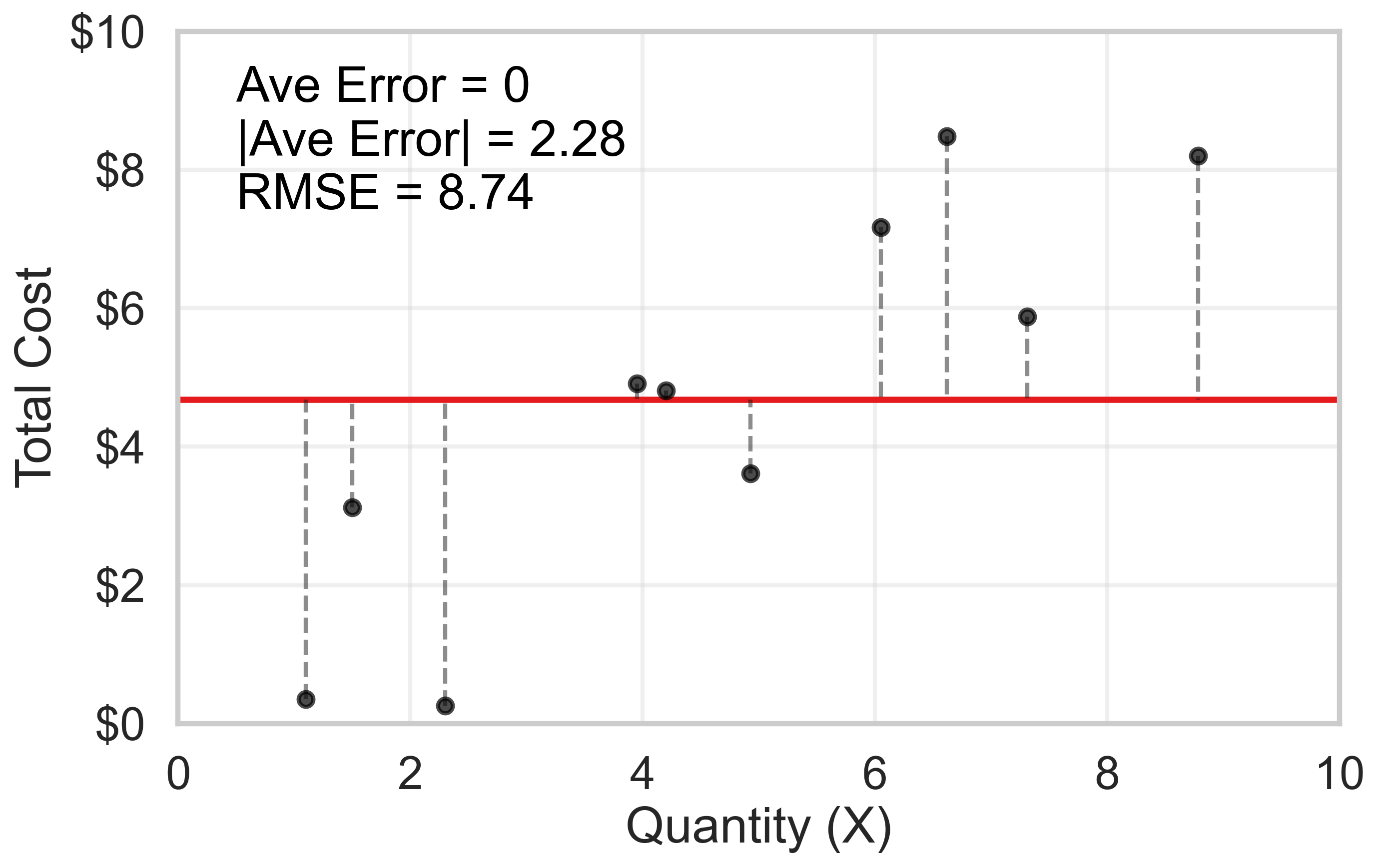
Fit the line by minimizing error
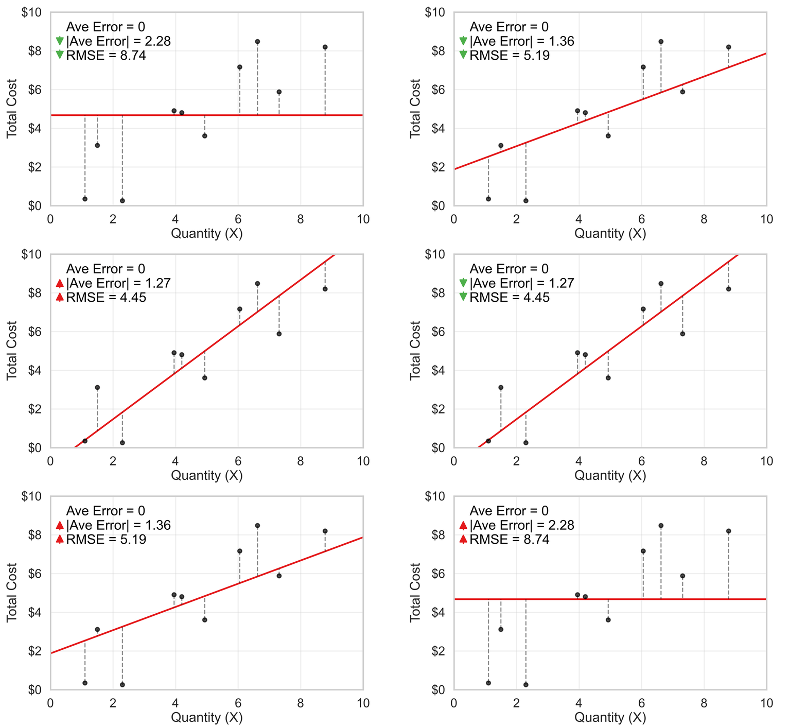
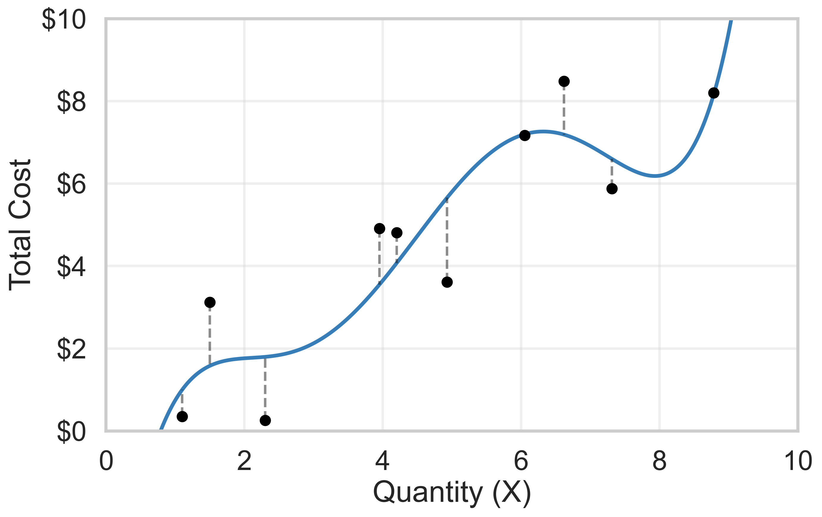
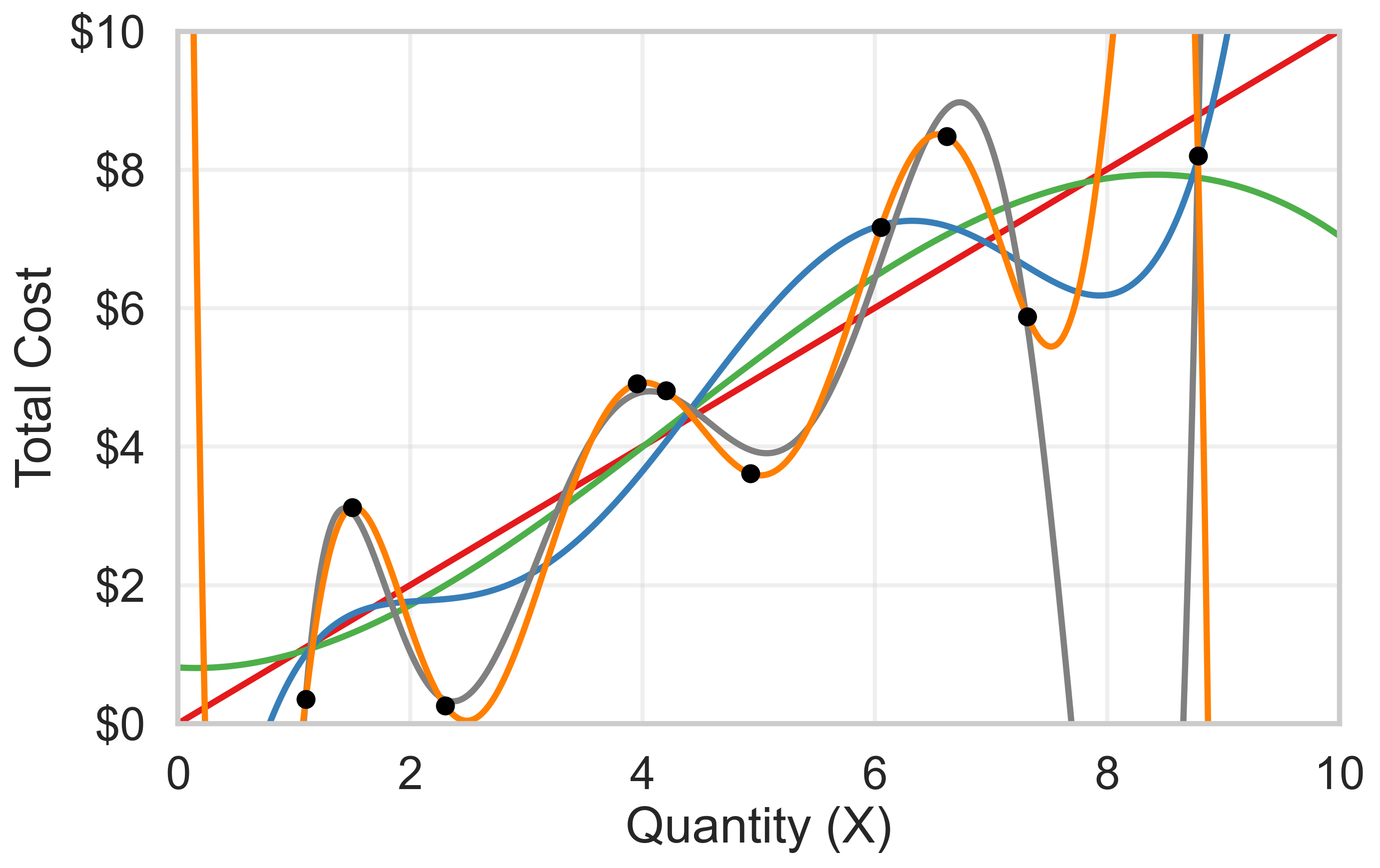
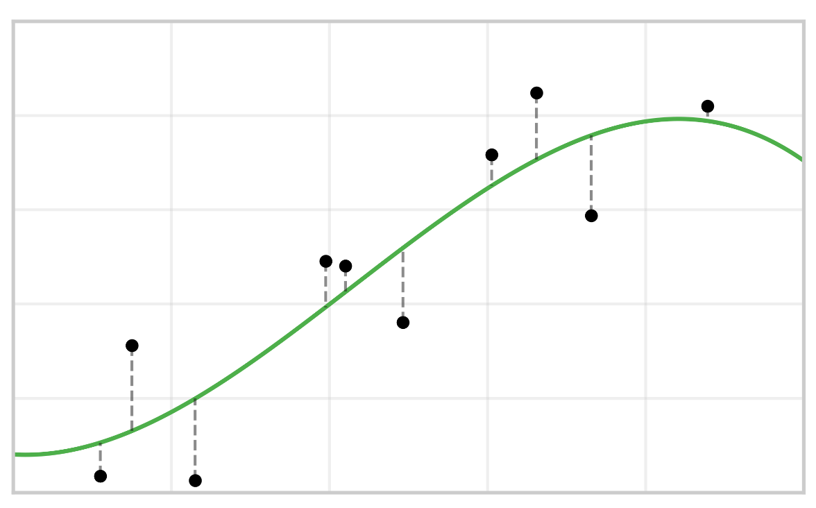
Fancier Regressions fit better
And better
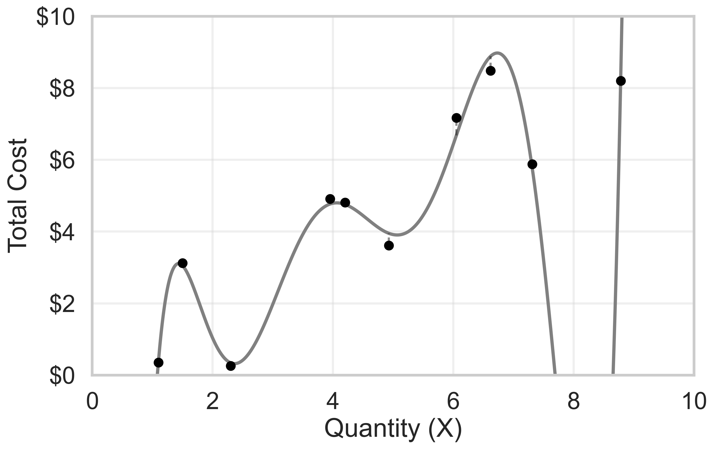
And better-ER
And Best-est
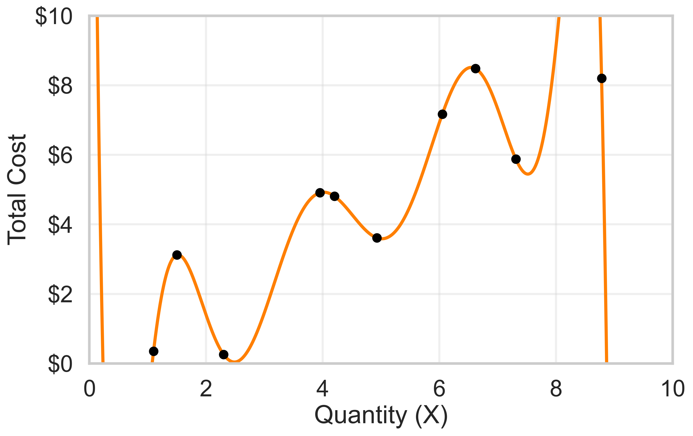
what’s the difference?
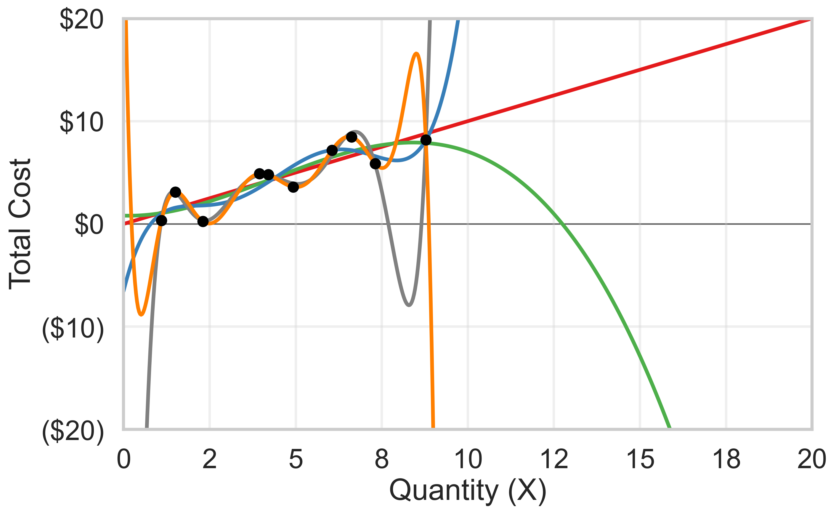
Why do we care?
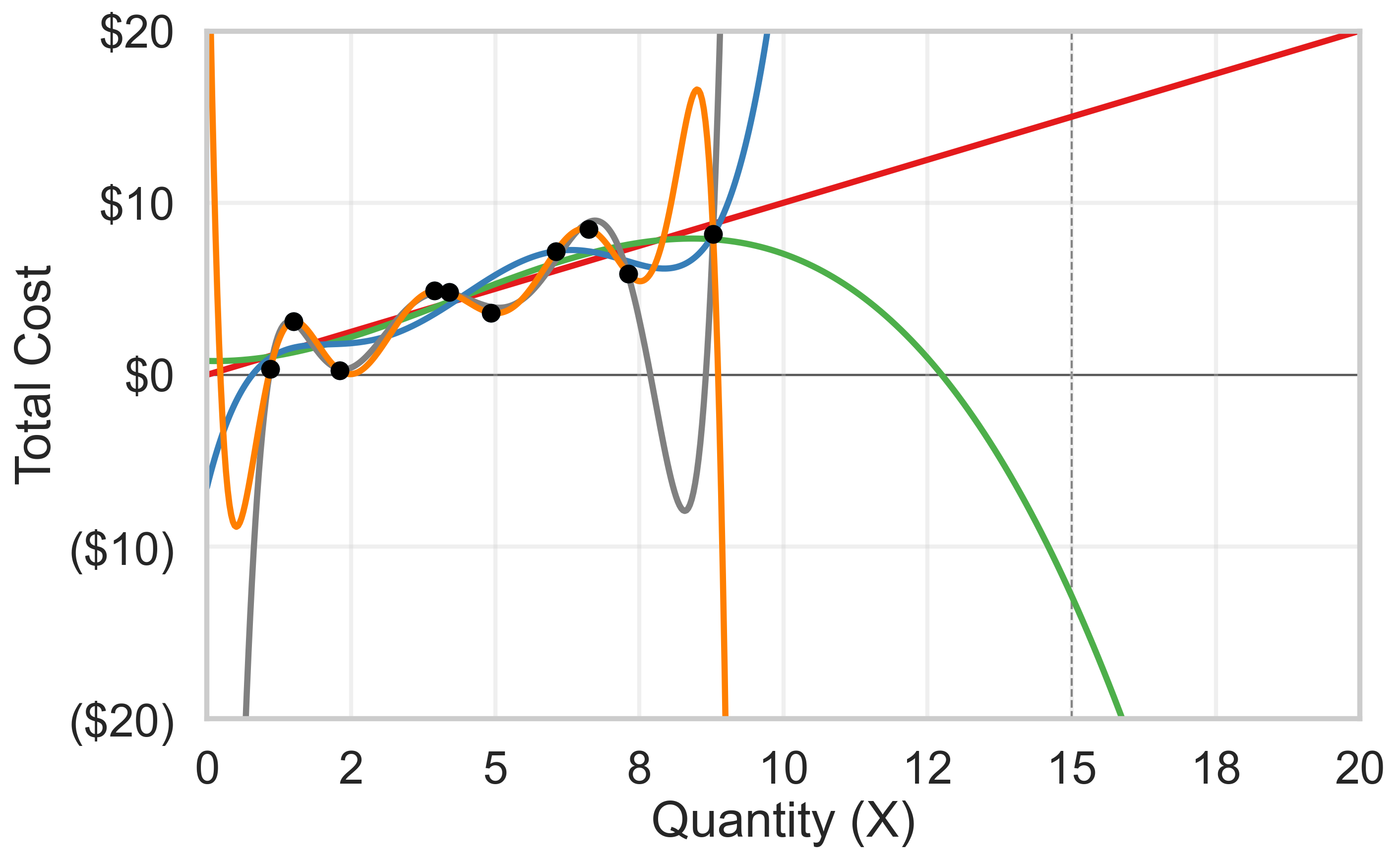
“Out of Sample” predictions
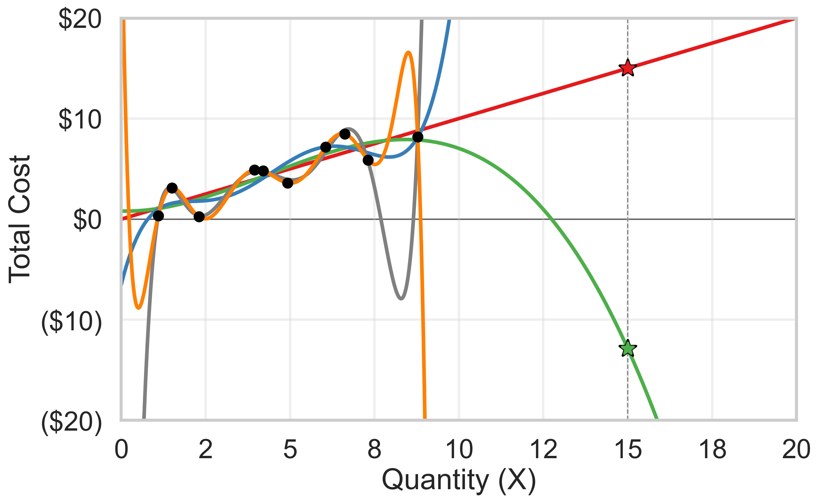
Regression Models
- Many different regression models
- Differ in assumptions
- Differ in data treatment
- Differ in treatment of model “error”
- Differ in what the analyst must specify
Most basic: OLS
- y = mx + b*
- Ordinary Least Squares – linear regression
- “Linear” in terms of inputs
- Very interpretable
- Requires feature engineering
- Vulnerable to outliers
Most basic: OLS
- y = mx + b*
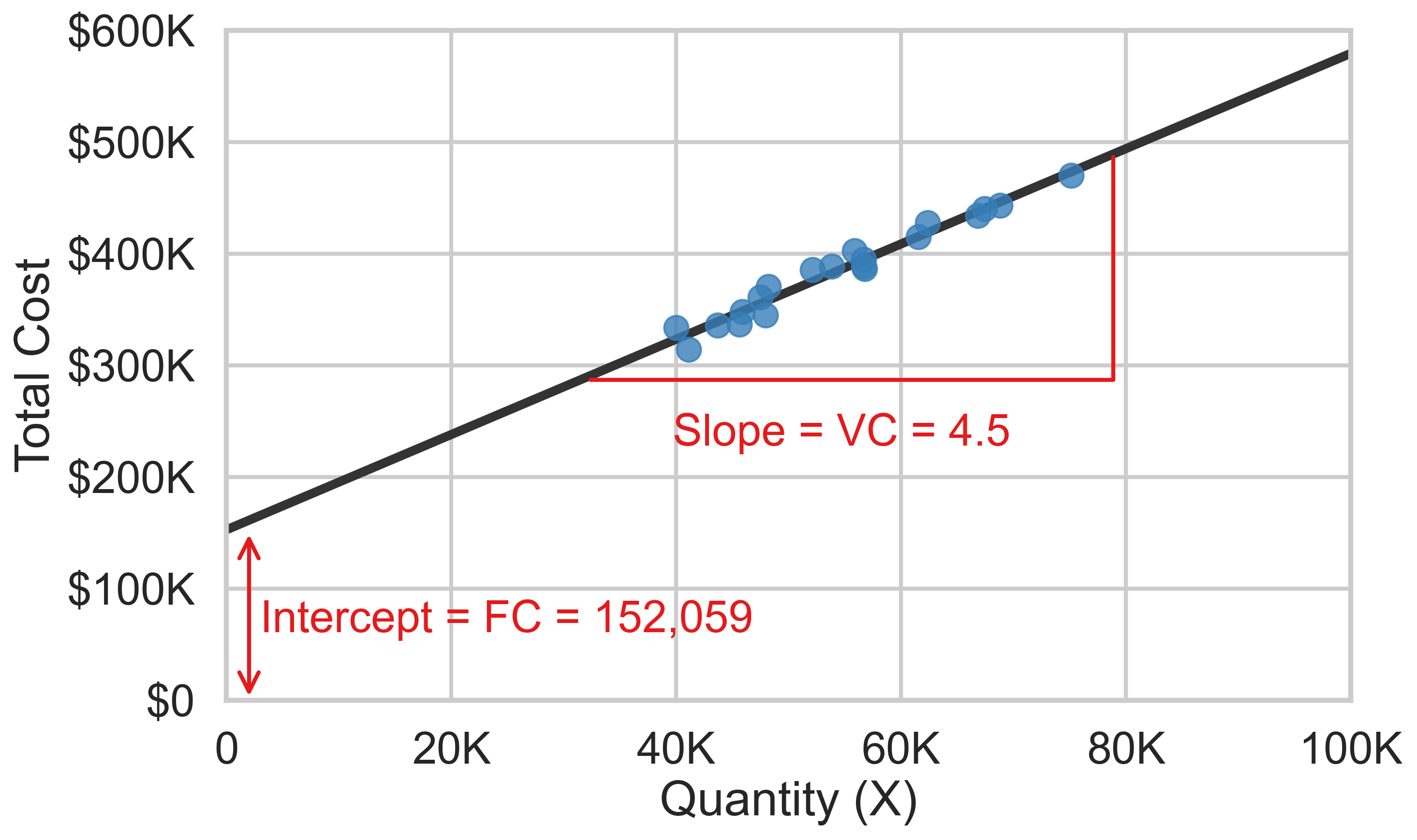
- Coefficients: when x changes by 1, y changes by m
Most basic: OLS
- y = mx + b*
- OLS computes “conditional mean,” or what would y be if x is ____.
- The variables are treated as independent
- Meaning if you put both height in inches and height in cm into the model, it wouldn’t know they are the same
Improving on OLS – extra-ordinary
- Add non-linearity for the x variables (polynomial)
- y = m1x + m2x2 + m3x3 + b*
- Add more or better x variables (multinomial)
- y = m1x + m2x + b
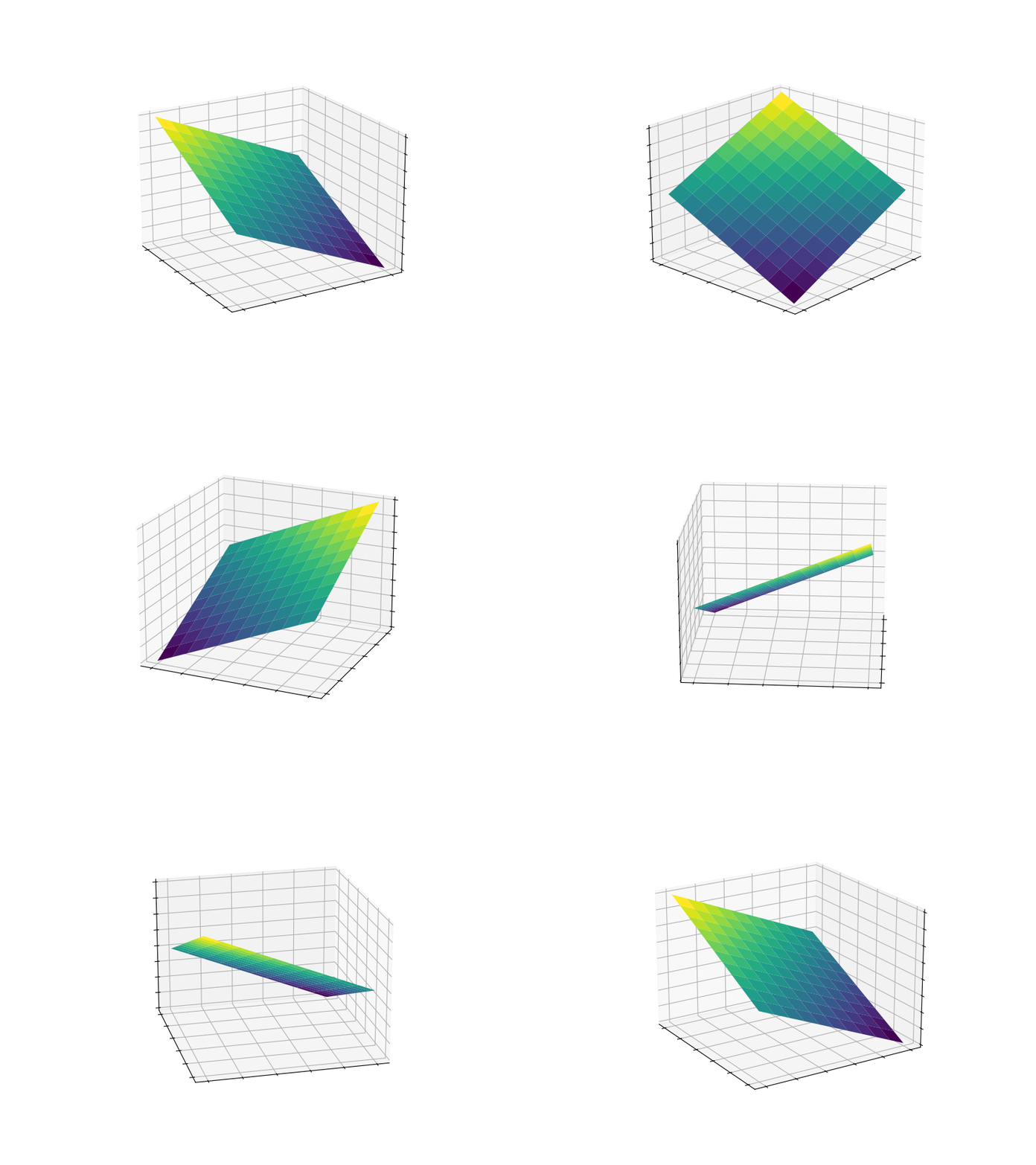
Fixed Effects
Fixed Effects
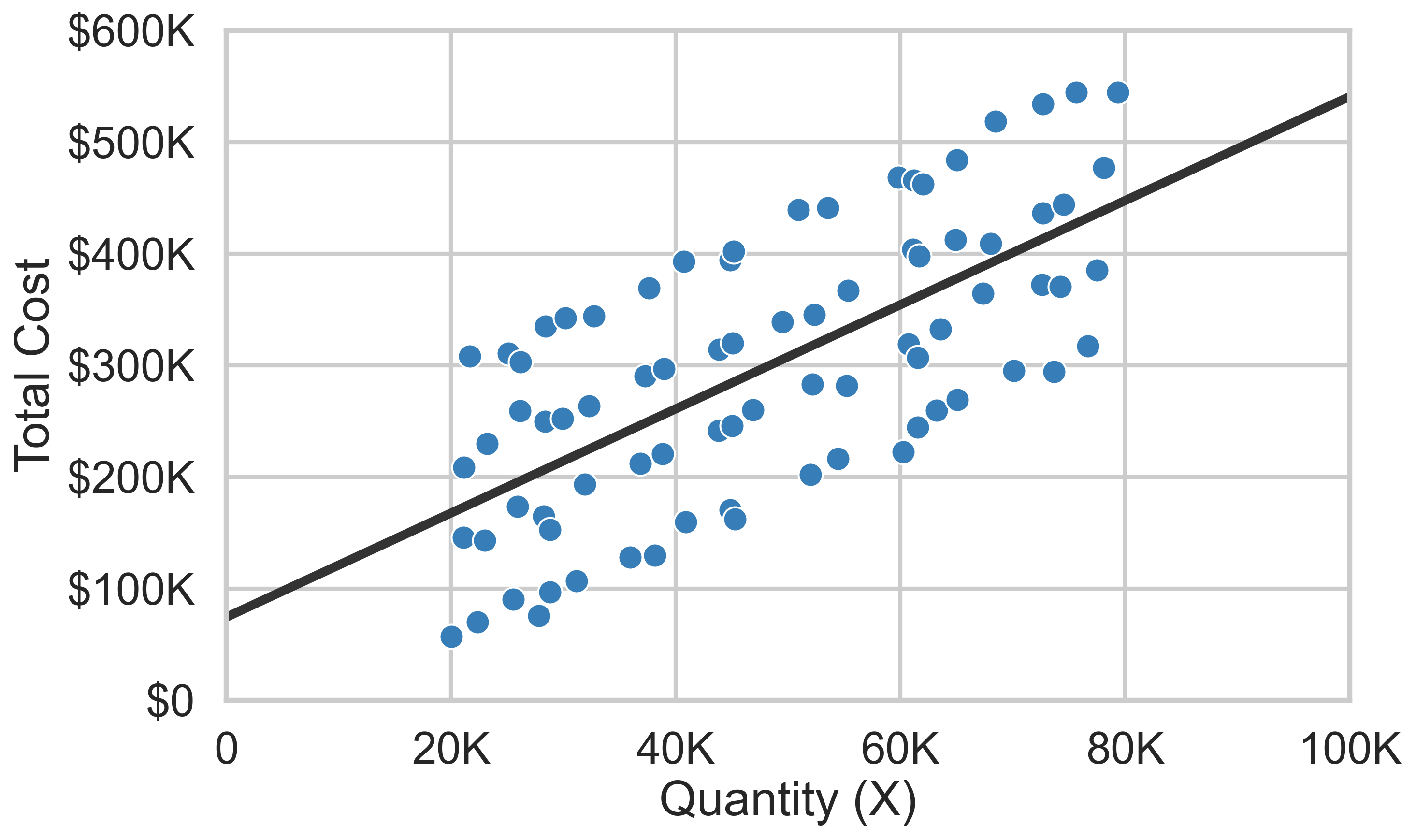
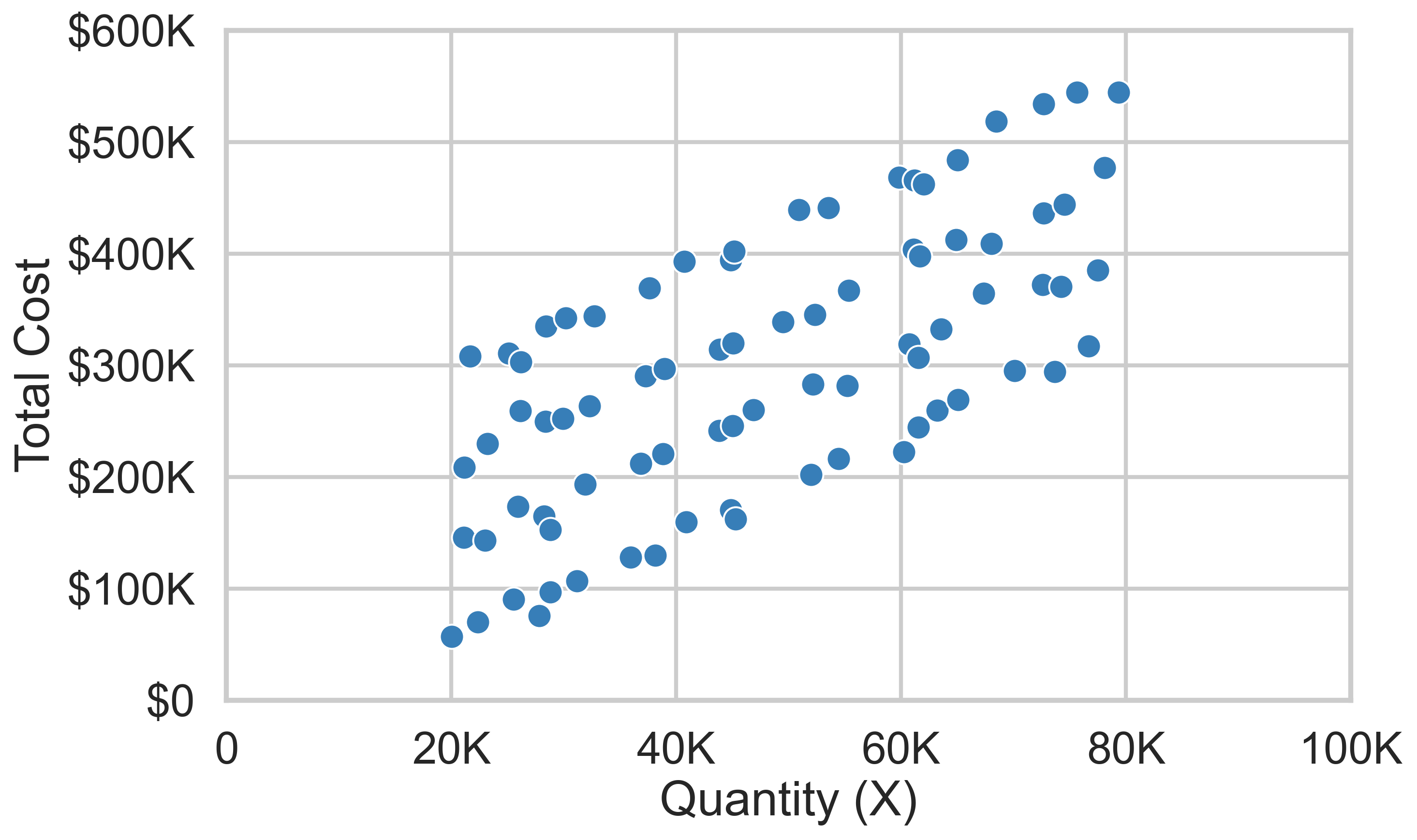
Fixed Effects
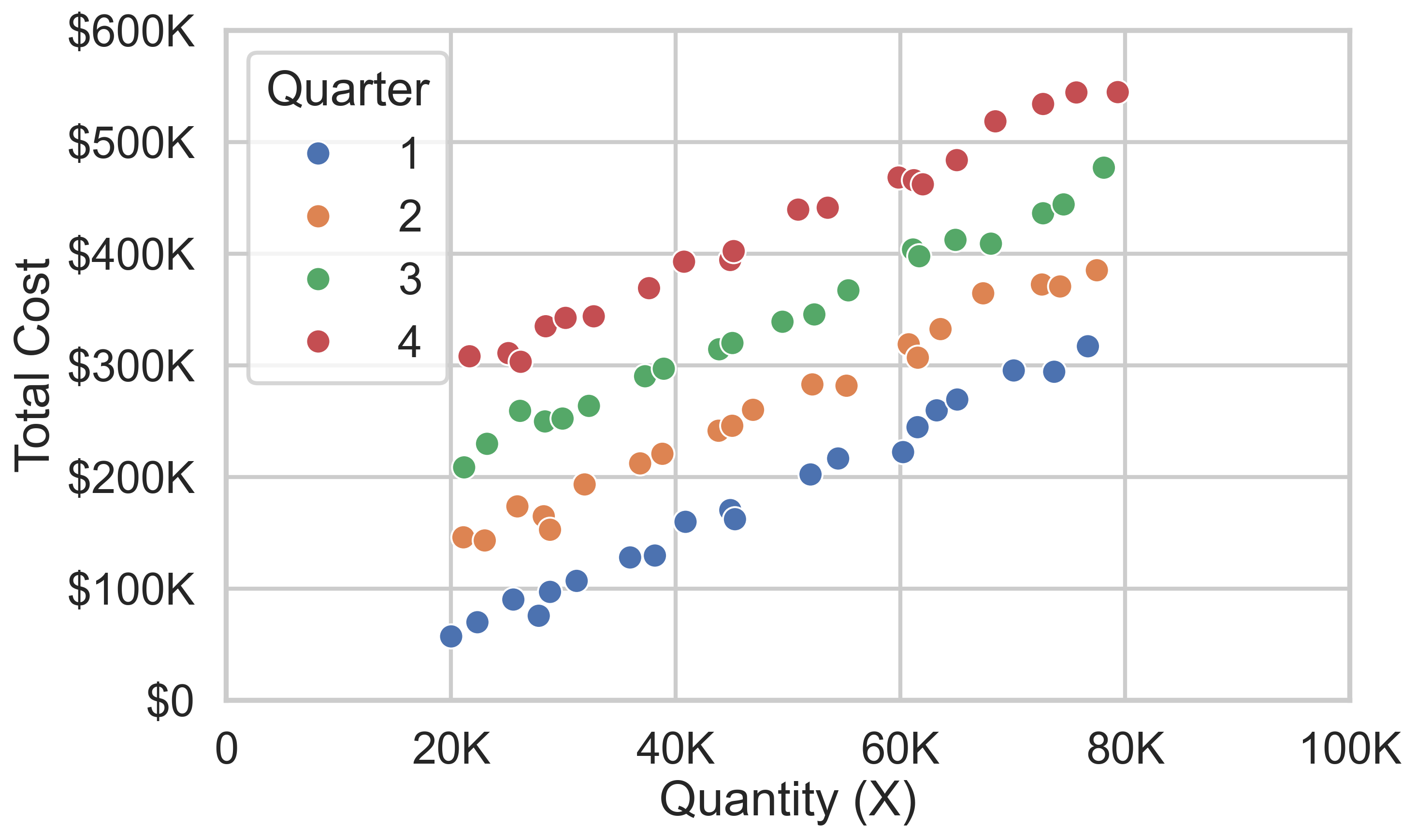
Fixed Effects
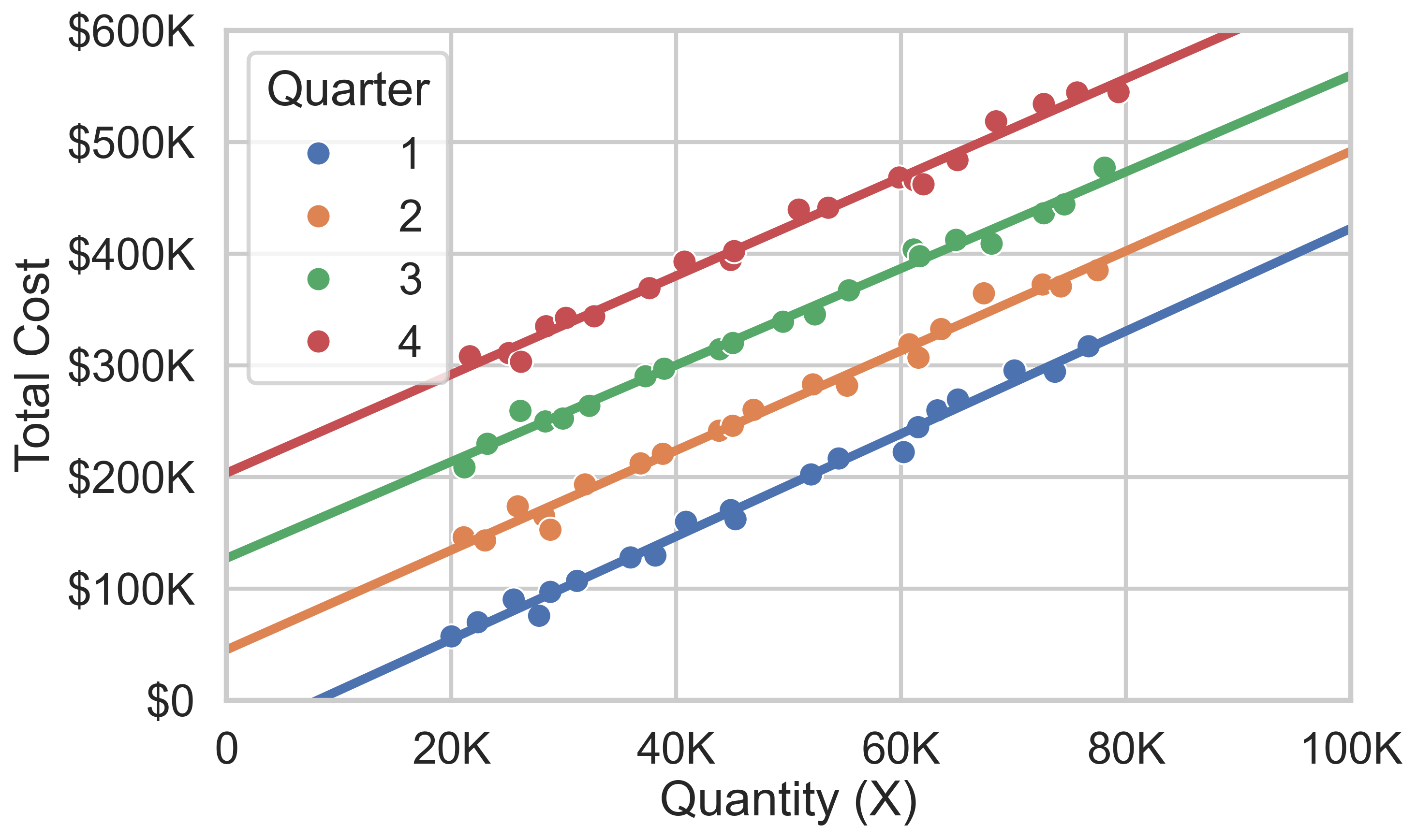
What to do with many x variables?
- We have to worry about “multicollinearity” which is jargon for x variables measuring the same thing
- Lasso/ridge regressions “penalize” the variables
- They have to be really important to not be eliminated
- We can use this to learn which variables matter most
- Dimensionality reduction (e.g., PCA)
Time-series data
- Each observation is related to the next
- Order matters
- Example: Revenue data over time
What do we use time-series for?
- Forecasting revenue, expenses
- Analyzing transaction trends over time
- Modeling crash risk, survival analysis
- Predicting demand for inventory management
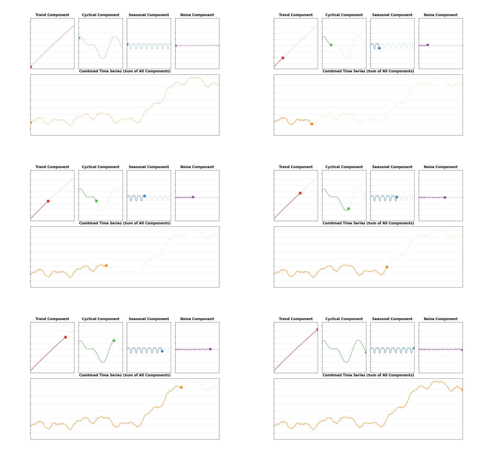
Components of time-series
- Trend
- Seasonal
- Cyclical
- Noise
Cautions
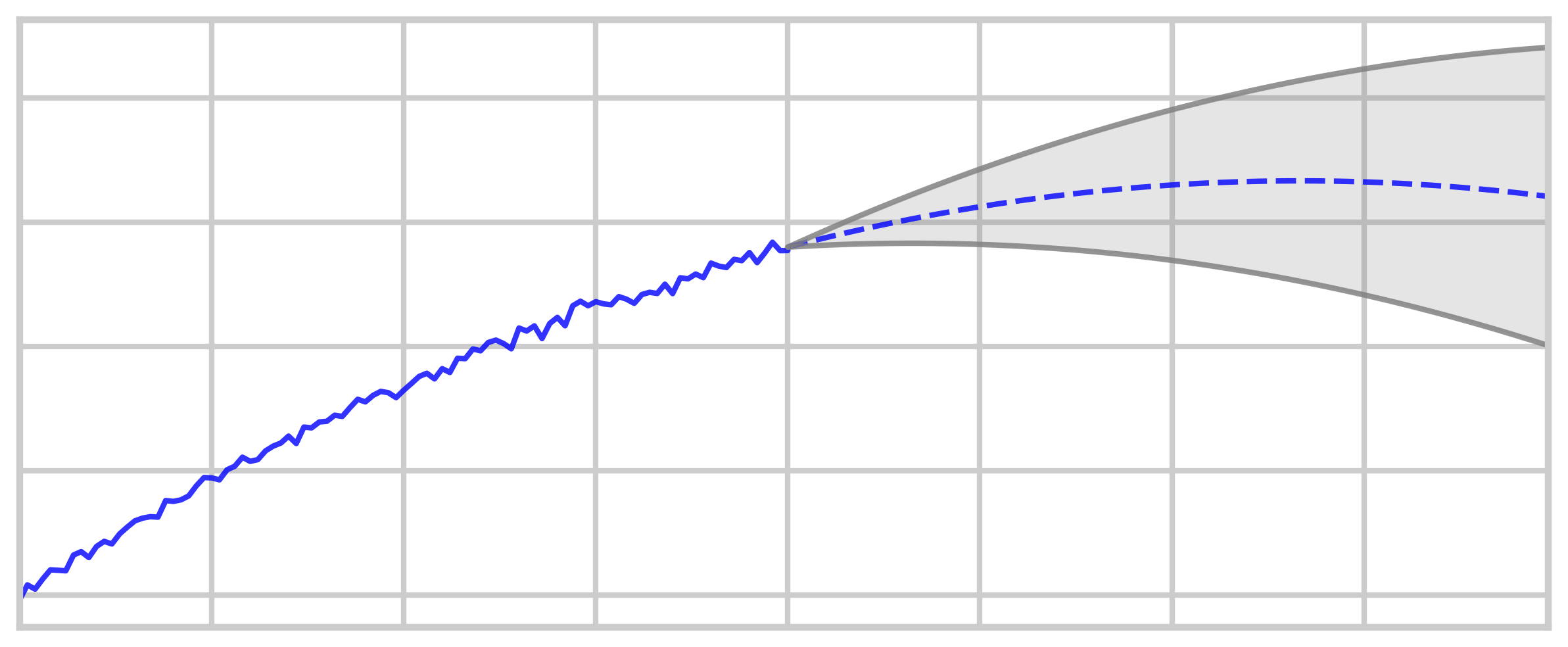
- Training data could contain random economic events that aren’t indicative of the future (overfitting)
- New economic events that aren’t modeled can occur (underfitting)
- Uncertainty increases when forecasting further out
Parametric vs Non-parametric
- Parametric models specify the relationships between variables and the outcome
- y = mx + b*
- Non-parametric doesn’t, just learns the best relationship it can
- y = f(x) + random error
- f is “learned” by predicting y as best as possible
Why add complexity?
- Complex patterns are hard to model
- When using multiple variables, they are often related
- Parametric methods require you to explicitly model these relations
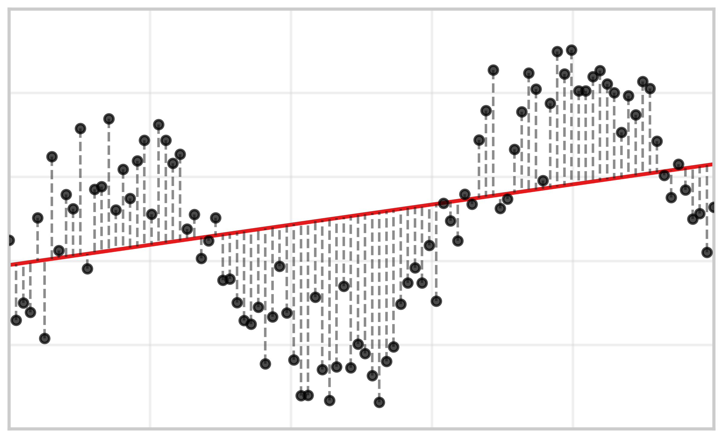
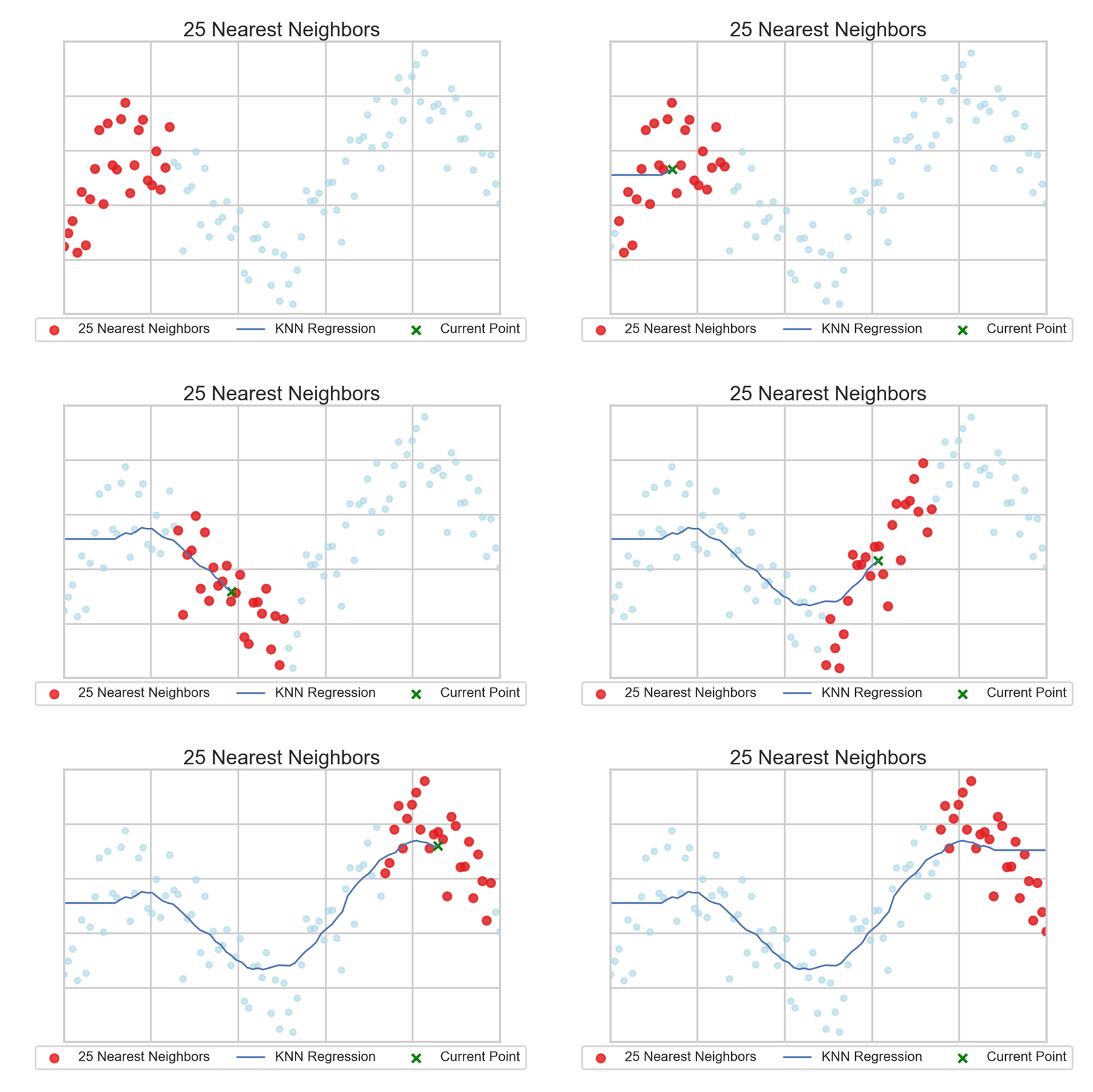
Local methods
- Examples: K-nearest neighbors, kernel regression
- Fit the line based on just the close points, not all
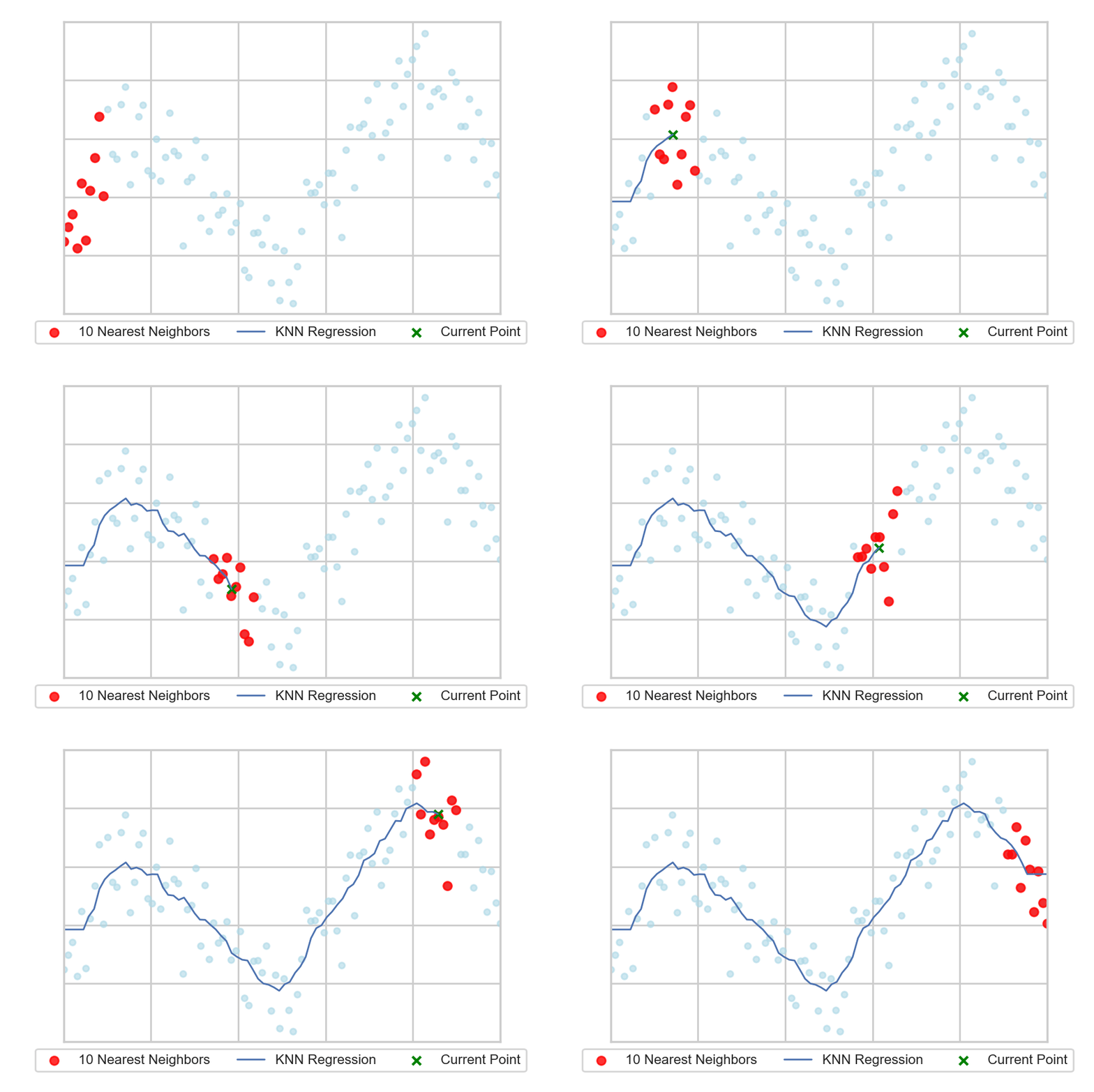
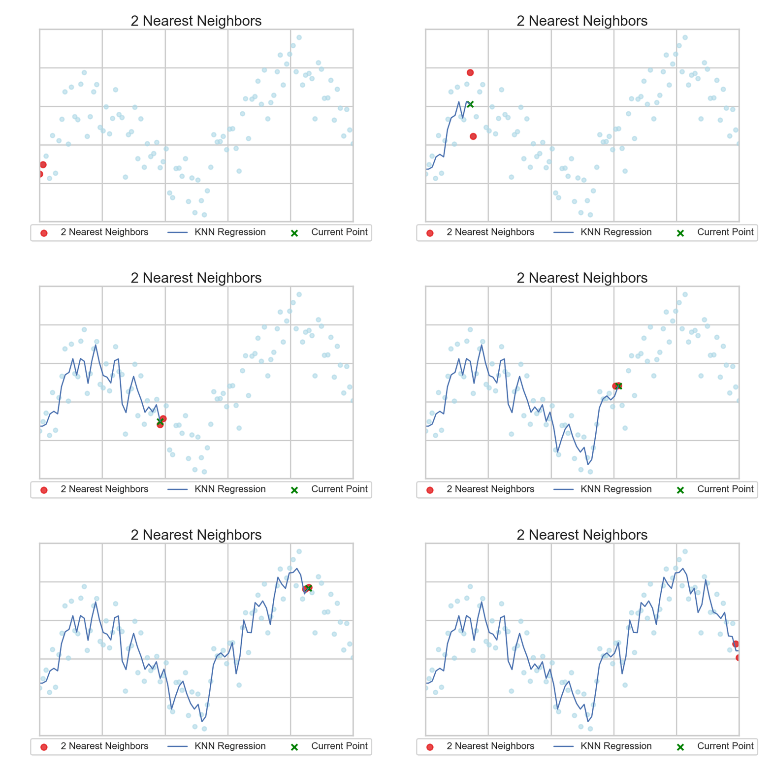
Local Methods
- Input from analyst is not the model, but “how” the algorithm should learn the line
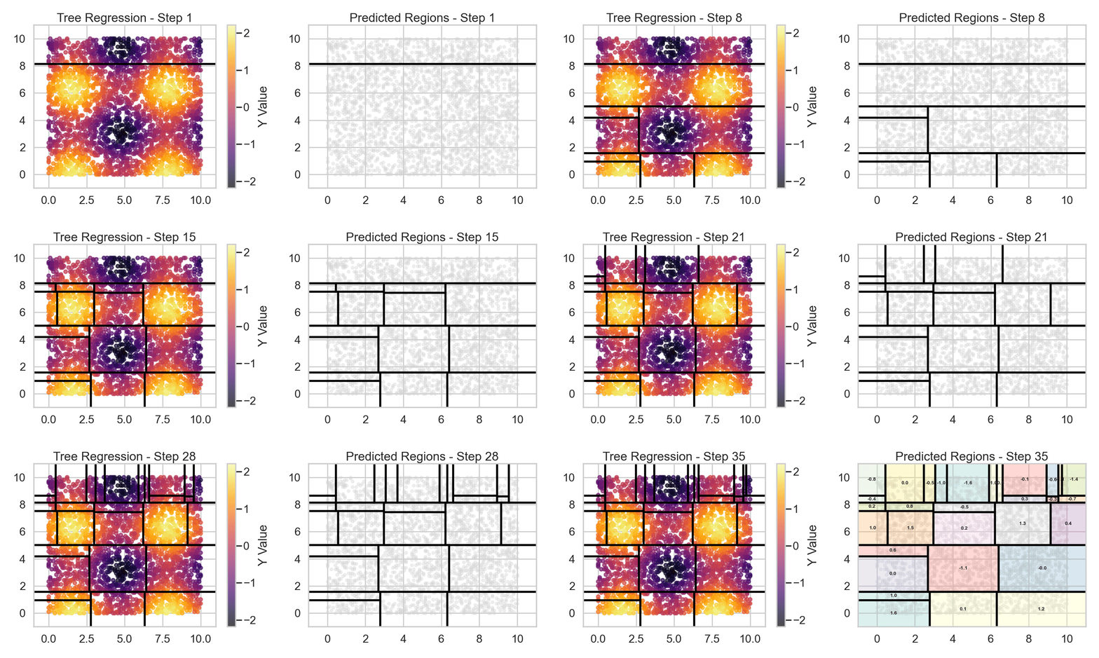
Tree-based models
- Decision tree regression is just a bunch of if-thens
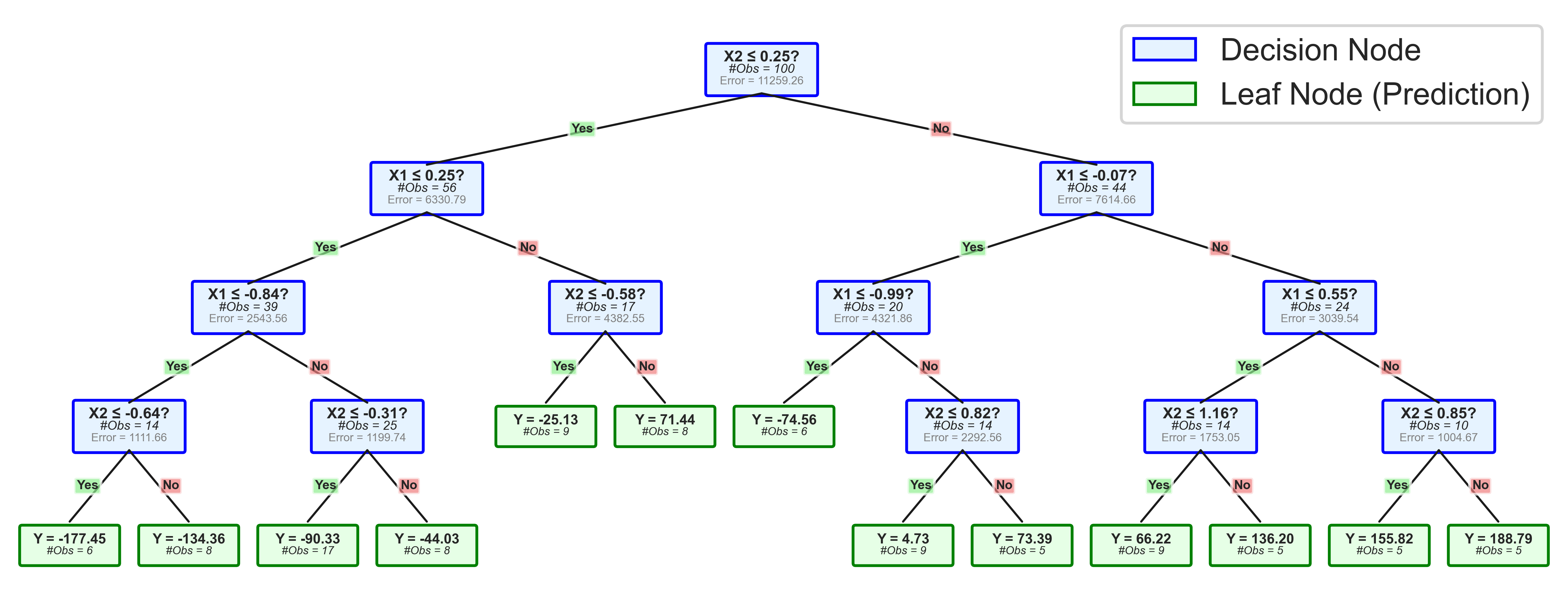
Tree-based models
When one tree isn’t enough
- Decision trees can overfit easily (more depth)
- Solution: combine multiple models into “ensembles”
- Take the average model output, or weight models based on accuracy
- Bagging: train on random data subsets (Random Forest)
- Boosting: train subsequent trees to fix errors (XGBoost)
- Stacking: trees on trees on trees (Neural Network)
In practice
- Start with XGBoost, if good enough, done
- Try other models if not
When to avoid more complex models
- If you know the real relationship, model it with a simple model!
- This will perform better out of sample, won’t overfit
- If you think the relationship is simple
- If you don’t have much data
- You need to interpretability
What is Causality
- Some outcome is the direct result of another action
- A directly causes Z
- A indirectly causes Z
Ice Cream Example
- Fact: Ice cream sales are positively associated with drowning rates
Ice Cream Example
- Fact: Ice cream sales are positively associated with drowning rates
- Causal: Ice cream causes drowning
Ice Cream Example

- Fact: Ice cream sales are positively associated with drowning rates
- Causal: Ice cream causes drowning
- Indirect causal: Ice cream causes drowsiness which leads to drowning
Ice Cream Example

- Fact: Ice cream sales are positively associated with drowning rates
- Causal: Ice cream causes drowning
- Indirect causal: Ice cream causes drowsiness which leads to drowning
- Reverse causal: drowning causes ice cream sales
Ice Cream Example

- Fact: Ice cream sales are positively associated with drowning rates
- Causal: Ice cream causes drowning
- Indirect causal: Ice cream causes drowsiness which leads to drowning
- Reverse causal: drowning causes ice cream sales
- Confounder (reality): Ice cream and swimming (thus drowning) both peak in the summer

Solution? Counterfactual!
- Jargon:
- Treatment: thing you’re studying the effect of (tax cut)
- Treated firms: firms that get the treatment (got tax cut)
- Control firms: firms that didn’t get treated (no tax cut)
- “Treatment Effect” is estimated effect of treatment
- = Outcometreated – Outcomecontrol
Solution? Counterfactual!
- Compare firm’s outcome when treatment occurs to that same firm’s outcome when treatment does not
- Outcome when treatment does not occur is called the “counterfactual”
- If firm is treated, how do we measure outcome when treatment does not occur (or vice versa)?
Common Counterfactuals
- Other firms that did not have treatment
- Randomized control trials (gold standard): randomly assign treatment to firms, so only difference is treatment
- Pseudo-experiments: find setting in which treatment occurring is effectively random (e.g. tax cut for firms > 1B)
- Same firm before treatment occurred
- Difference in difference: both of the above
- Note: all these are estimated as averages across firms
Difference in Difference
- Looking at firm’s change due to treatment isn’t enough if untreated firms also changed
- Example:
- Firms that got PPP loans saw huge declines in sales
- So PPP loans caused loss in sales?
- Firms that did not get PPP loans saw larger losses
- Compared to counterfactual, firms with PPP loans had relatively higher sales (but still lower then w/o Covid)
Caveats and Concerns
- It all comes down to how good your counterfactual is
- Anything that is different between treatment and control could potentially cause the estimated effect
- Called omitted variables or measurement error
- Solutions to identify causality limit generalizability
- If you can’t define how treatment results in outcome (the mechanism), be very skeptical
- If you can, then that’s potentially testable
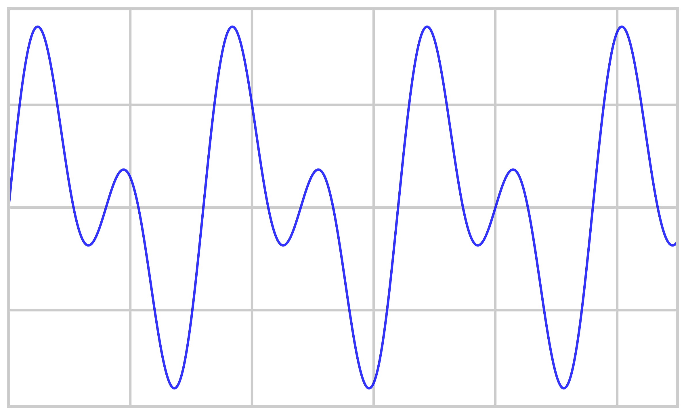
Stationarity
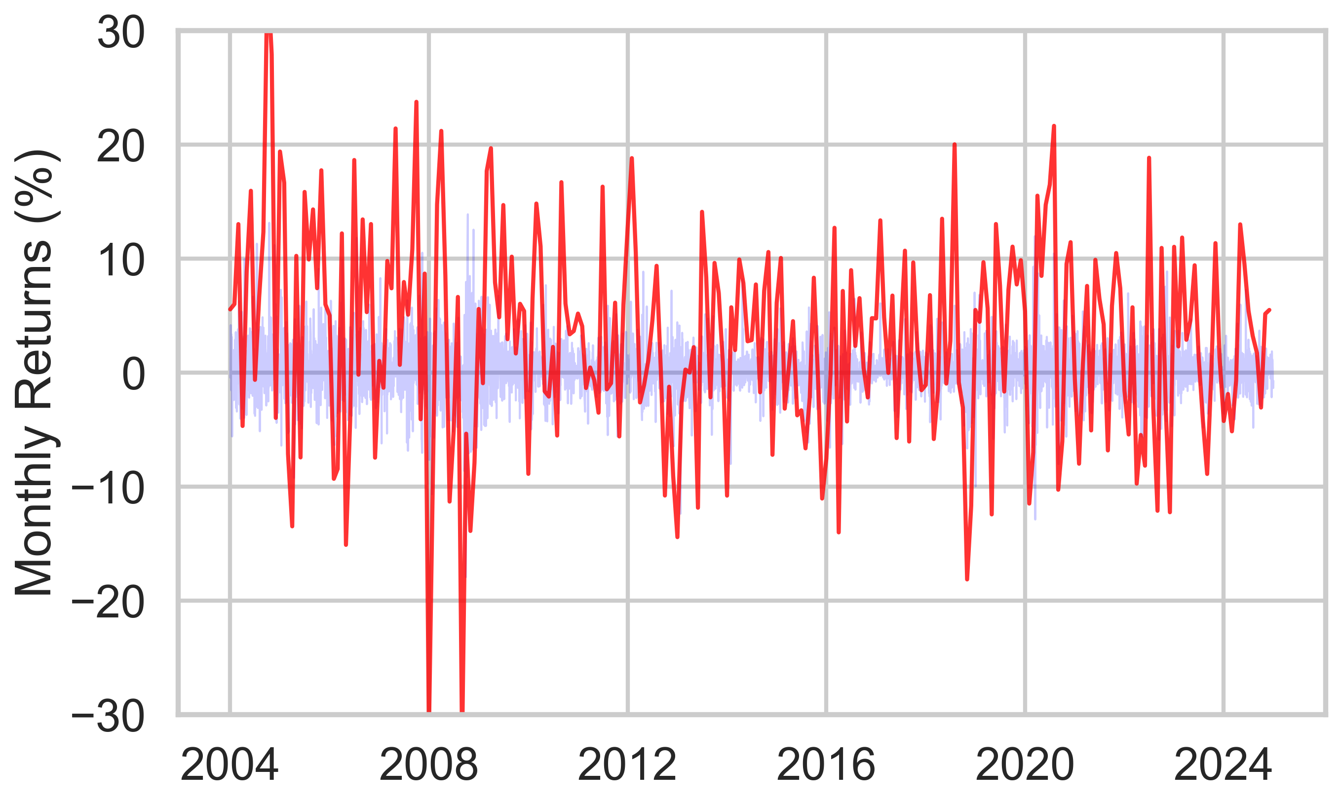
- A stationary process stays in the “same place”
- Statistics about the data behave nicely
Stationarity
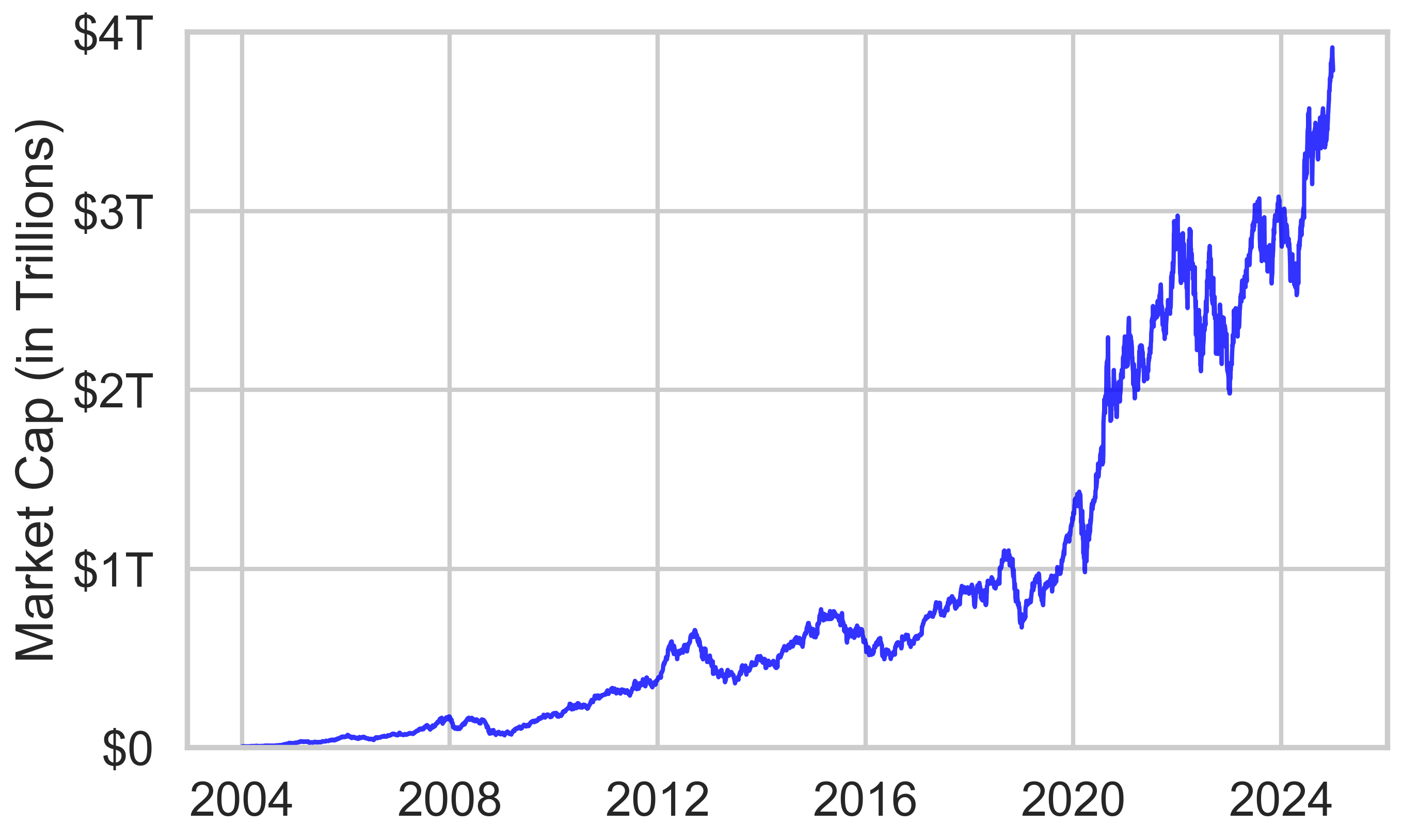
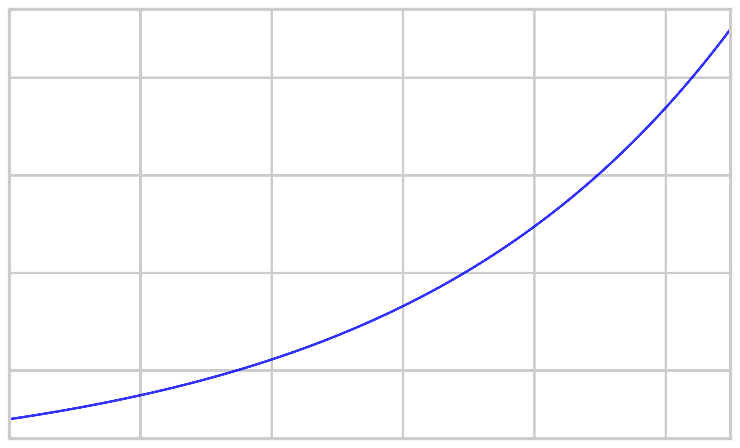
- A non-stationary process “moves” too much
- Statistics about the data behave poorly (meaningless?)
Stationarity – So what?
- Analytics on a non-stationary will often be wrong
- A non-stationary process needs different math
- A non-stationary process could be “made” stationary
- This is why we often study returns, not market cap