Lab 1: Opening Software
Lab 1 will be an overview of the main tools we will use for completing the labs: Microsoft Excel and Python. This initial lab is designed to ensure you can access and open a dataset in each environment. We will perform the same basic task of opening a data file on both platforms to get a very preliminary familiarity with each tool.
Assignment Notes
Learning Objectives
By the end of this lab, you will be able to:
- Successfully download a dataset and locate it on your computer.
- Open and view a data file in Microsoft Excel (using Power Query) and a Python Jupyter Notebook.
- Begin to understand the differences between each piece of software, their strengths, and weaknesses.
Submission Expectations
- Submit screenshots demonstrating successful loading of data in the two modalities described below.
Rubric and Grading
- For Lab 1, on-time submission of screenshots of both modalities will get full marks.
A Note on Platforms (Windows, macOS, Linux)
Both tools are available in desktop form on Windows and macOS, while (I believe) only Python is available on Linux. Both are available online/cloud-based as well. My intent is that these labs can be completed on any machine. If you find this isn’t the case, or if you find an issue related to operating systems, please let me know!
Data
The dataset we will be opening in both tools is a Tab-Separated Value file containing journal entry line items. This is a common format for exporting data from accounting systems.
The file is named JEA Detail.txt (link). It is a made up company’s 2024 rent expense detail (the file came from EYARC, credit to the EY team!).
Note: A few things in this file should look wrong: quoted numbers, spacing, etc. That is not a mistake in your download, it is what a real system might export. Cleaning this up is the whole point of Lab 2. For Lab 1, all you need to do is get the file open.
How-to Steps
The following outline how to perform the lab in each modality.
Step 0 - Set up class folder
Before we dive into the data, take a moment to set up your digital workspace. Good data science hygiene starts with organization. Think of your file structure as a Lab Notebook, whose purpose is:
- Reproducibility: You (or anyone else) should be able to re-run your analysis later. Keeping data and analysis together is step one.
- Documentation: Clear structure helps you remember what you did weeks or months from now.
- Sanity: Separating tasks prevents files from getting mixed up and overwritten.
While this is entirely optional (it’s your computer!), I suggest:
- Create a main class folder: somewhere on your computer (e.g.,
Documents/ACCT_5150), create a folder for this course. - Create a lab folder: Inside that class folder, create a new sub-folder named
Lab_1. - Download data to this folder: Move the
JEA Detail.txtfile you downloaded into thisLab_1folder.
Step 1 - Excel (Power Query)
The first software will be Excel. Instead of simply opening the file, we will use Power Query to import the data. This is a powerful feature that creates a connection to your data source. This means if you update the data file (e.g., replace it with new data), you can simply “refresh” your Excel model to update the analysis automatically, without re-doing your work.
- Open Excel: Open a blank Excel workbook.
- Import data:
- Go to the Data tab on the ribbon.
- Click
Get Data>From File>From Text/CSV. - Navigate to where you saved
JEA Detail.txtand select it. Click Import.
- Load data:
- A preview window will appear. Ensure the Delimiter is set to Tab (Excel usually detects this automatically).
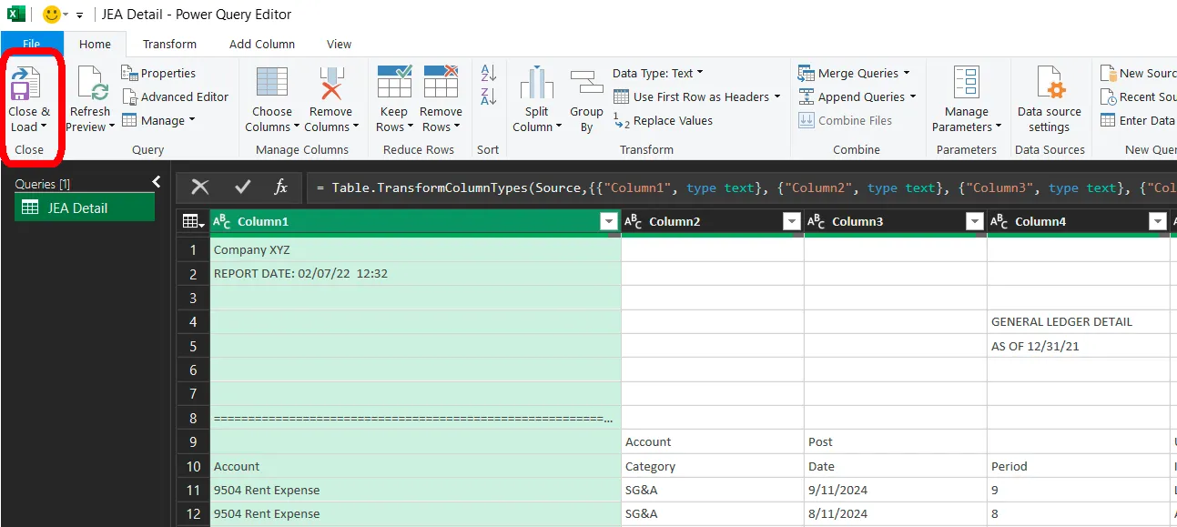
- Click Transform Data. This opens the Power Query Editor, where you can perform data transformations. You can also open the Power Query Editor directly, then add the data by clicking
New Source>File>From Text/CSV.
- Load data into sheet: Later, we will use this Power Query window to perform some cleaning/transforms, but for now that’s all we need. Click “Close & Load” to load the data into a sheet (see screenshot below).
- Save: Save your workbook as
Lab1_Excel.xlsx. - Screenshot: Take a screenshot of the data open in Excel (showing the table loaded from Power Query, often defaults to green striped rows).
Step 2 - Python
The second software will be Python. We will primarily use Google Colaboratory (Colab), a free, cloud-based Jupyter Notebook environment that requires no local installation.
Option A: Google Colab (Cloud)
- Go to Google Colab: Navigate to colab.research.google.com. Log in with your University Google account ([uID]@gcloud.utah.edu) or a personal one. Logging in means that the notebooks you create will be saved to your Google Drive.
- Create a notebook: Click
File>New notebook. - Link to Google Drive (recommended):
By default, Colab files are temporary. To save your work and data persistently:
- Click the “Mount Drive” button in the top-left corner of the Colab interface, or run this code cell to mount your Drive:
from google.colab import drive drive.mount('/content/drive') - Follow the prompts to authorize.
- You can now access your files at
/content/drive/MyDrive/. I suggest creating a folder there for this class (e.g.ACCT_5150, which will then be/content/drive/MyDrive/ACCT_5150).
- Click the “Mount Drive” button in the top-left corner of the Colab interface, or run this code cell to mount your Drive:
- Upload/access data:
- If using Drive: Upload the
JEA Detail.txtfile to your Drive folder, then find it in the Colab file pane (left side, folder icon > drive > MyDrive). Right-click the file and “Copy path”. - If not using Drive: Click the folder icon on the left, then the upload icon (page with arrow) to upload
JEA Detail.txtto the temporary session storage.
- If using Drive: Upload the
- Load data with Pandas:
import pandas as pd # Use the path you copied or just the filename if uploaded directly file_path = "JEA Detail.txt" # or "/content/drive/MyDrive/ACCT_5150/JEA Detail.txt" # Note: We use sep='\t' because it is a Tab-Separated Value file df = pd.read_csv(file_path, sep='\t') - View data:
Run the cell to see the first 5 rows.df.head() - Screenshot: Take a screenshot of the data open in Colab (showing the table displayed after the
df.head()cell).
Option B: Local Installation (Miniconda)
If you prefer to run Python locally (platform agnostic), Miniconda is recommended.
- Install Miniconda: Download/install from docs.conda.io.
- Create environment: Open your terminal/Powershell and run:
conda create -n analytics python pandas jupyter conda activate analytics - Run Jupyter:
This opens a local notebook interface in your browser.jupyter notebook - Create a notebook: In the Jupyter interface, click “New” > “Python 3” (or “Notebook”) to create a new notebook file (
.ipynb). - Load data with Pandas:
import pandas as pd # Use the path you copied or just the filename if your notebook is in the same folder as the data file_path = "JEA Detail.txt" # Note: We use sep='\t' because it is a Tab-Separated Value file df = pd.read_csv(file_path, sep='\t') - View data:
Run the cell to see the first 5 rows.df.head() - Screenshot: Take a screenshot of the data, showing the table displayed after the
df.head()cell.
Tip: For the local option, I would strongly recommend using VSCode, and installing the Python extension. This will greatly simplify the process of running Jupyter notebooks, as you can natively open the notebook file in VSCode and run it from there.
Submission
To complete this lab, you will provide evidence that you have successfully opened the data file in both tools.
-
Take screenshots:
- Capture a screenshot of the data open in Excel (showing the green table from Power Query).
- Capture a screenshot of your Google Colab (or local Jupyter) notebook showing the output of the
df.head()command.
Screen-capture notes:
- Windows Note: To take a screenshot on Windows, press
Win + Shift + sand then click-and-drag a rectangle to capture that portion of your screen (to grab the full screen, hitPrtScon the keyboard, orAlt + PrtScto capture just the current window). - macOS Note: To take a screenshot on macOS,
Shift + Command + 5will open the screenshot app, which is nice, orShift + Command + 4will let you click-and-drag a rectangle to capture that portion of your screen (which I believe saves the screenshot to a file, but I don’t know where? If you want to just copy the screen to your clipboard for pasting into word/Google Docs, add Control, soControl + Shift + Command + 4).
-
Submit to Canvas:
- Navigate to the Lab 1 assignment on Canvas and upload your screenshots.